DDPM 原理推导

文章基本信息

• 文章名称：Denoising Diffusion Probabilistic Models
• 发表会议/年份：NeurIPS 2020
• 作者：Jonathan Ho, Ajay Jain, Pieter Abbeel
• 单位：UC Berkeley

前置知识

1. Markov：当前位置的概率只会受到前一时刻概率影响
2. 正态分布的叠加性$eg. N(\mu_1,\sigma_1^2)+N(\mu_2,\sigma_2^2) = N(\mu_1+\mu_2,\sigma_1^2+\sigma_2^2)$
3. 贝叶斯：$P(A|B) = \frac{P(B|A)P(A)}{P(B)}$,$P(A|B,C) = \frac{P(B|A,C)P(A|C)}{P(B|C)}$

开始推理

前向过程

我们定义每次加入的噪声是一个正态分布，满足如下式子：

$$q(x_t|x_{t-1}) = \mathcal{N}(x_t; \sqrt{\alpha_t} x_{t-1}, \beta_t I)$$

在DDPM（Denoising Diffusion Probabilistic Models）中，这个公式表示从时间步骤 $t-1$ 到时间步骤 $t$ 的状态转移概率。具体来说，$q(x_t | x_{t-1})$ 表示给定前一状态 $x_{t-1}$ 时，状态 $x_t$ 的概率分布。

符号 $\mathcal{N}$ 表示高斯（正态）分布，$\sqrt{\alpha_t} x_{t-1}$ 是该高斯分布的均值，而$\beta_t I$ 是分布的协方差，这里 $\alpha_t$ 和 $\beta_t$ 是与时间步骤 $t$ 相关的系数，$I$ 是单位矩阵，表示协方差矩阵是对角的。

在DDPM中，这个过程通常被用来逐步增加数据的噪声，其中 $\alpha_t$ 和 $\beta_t$ 是随时间变化的，通常是减小的，这样随着时间的推移，生成的样本会越来越多地偏离初始样本的分布。简而言之，DDPM的核心是一系列的噪声添加和去噪步骤，该公式描述的是其中噪声添加过程的概率分布。

$$x_t = \sqrt{\alpha_t} x_{t-1} + \sqrt{\beta_t}\epsilon_t \quad \epsilon_t \sim \mathcal{N}(0, I)$$

$$\alpha_t = 1-\beta_t$$

我们可以将递归式展开，变为直接$O(1)$计算到任意时间点的正向加噪结果

$$\begin{align*} x_t &= \alpha_t x_{t-1} + \beta_t \epsilon_t \\ &= \alpha_t (\alpha_{t-1}x_{t-2} + \beta_{t-1}\epsilon_{t-1}) + \beta_t \epsilon_t \\ &= \cdots \\ &= (\alpha_t \cdots \alpha_1)x_0 + \underbrace{(\alpha_t \cdots \alpha_2)\beta_1\epsilon_1 + (\alpha_t \cdots \alpha_3)\beta_2\epsilon_2 + \cdots + \alpha_t \beta_{t-1}\epsilon_{t-1} + \beta_t \epsilon_t}_{\mathcal{N}(0, (1-\alpha_t^2 \cdots \alpha_2^2)I)} \end{align*}$$

我们设:$\overline{\alpha}_t=\alpha_1\cdots \alpha_t$

化简上式可得：

$$q(x_t|x_0) = \sqrt{\overline{\alpha}_t}x_0+\sqrt{1-\overline{\alpha}_t}\epsilon\quad\epsilon\sim\mathcal{N}(0,I)$$

$$q(x_t|x_0) = \mathcal{N}(x_t; \sqrt{\overline\alpha_t} x_0, (1 - \overline\alpha_t)I)$$

这里 $\epsilon$ 是另一个服从 $\mathcal{N}(0, 1)$ 的分布，以上便是前向过程涉及到的公式推理

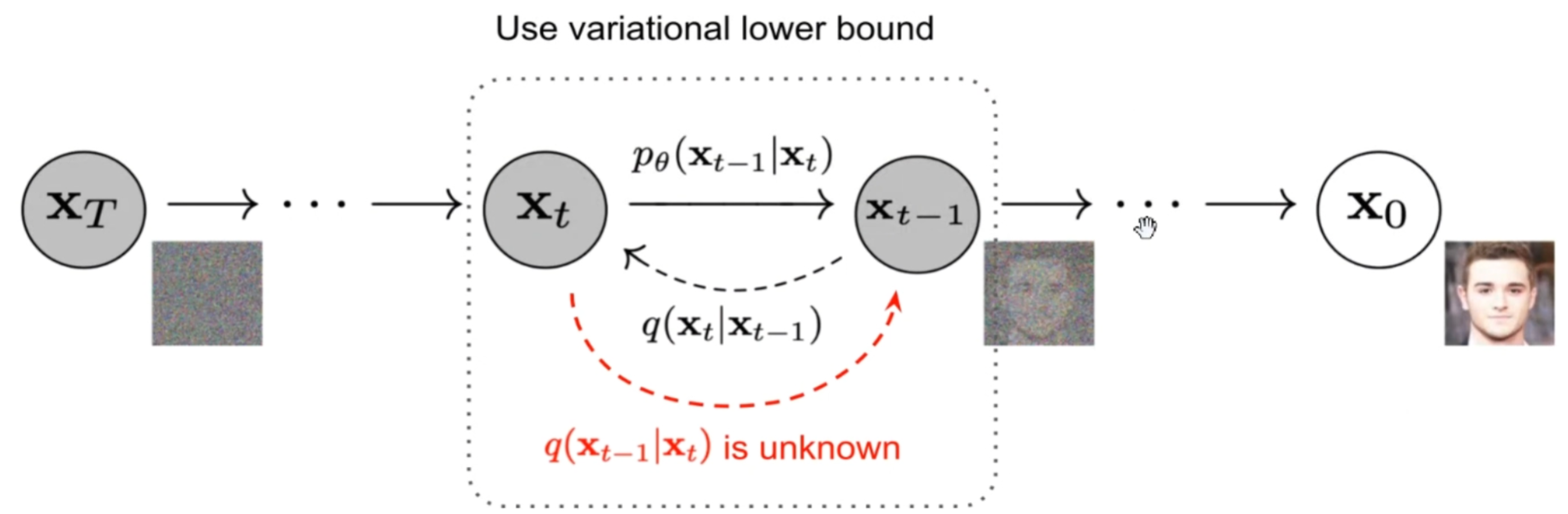
逆向过程

逆向过程又称去噪过程，之前的前向过程是给定$x_0$求任何时候的$x_t$即$q(x_t|x_0)$，那么去噪过程所求的分布就是给定任意时刻的分布$x_t$求初始分布$x_0$,即$p(x_0|x_t)$,通过马尔可夫假设，我们可以对逆向过程进行化简：

$$p(x_0 | x_t) = p(x_0 | x_1)p(x_1 | x_2) \cdots p(x_{t-1} | x_t) = \prod_{i=0}^{t-1} p(x_i | x_{i+1})$$

那如何求解$p(x_{t-1}|x_t)$呢，前面的加噪过程我们已经推出了$q(x_t|x_{t-1})$,我们可以通过贝叶斯公式把它们利用起来：

$$p(x_{t-1}|x_t) = \frac{p(x_t|x_{t-1})p(x_{t-1})}{p(x_t)}$$

注意：这里的(去噪)p和上面的(加噪)q只是对分布的一种符号记法,它们是等价的.

然后就又有一个新的问题，$p(x_{t-1})$和$p(x_t)$是未知的，但根据之前的正向过程推到，我们是知道$p(x_{t-1}|x_0)$以及$p(x_t|x_0)$,因此下面的式子我们是可以推出的。

$$p(x_{t-1} | x_t, x_0) = \frac{p(x_t | x_{t-1}, x_0) p(x_{t-1} | x_0)}{p(x_t | x_0)}$$

因为我们定义了DDPM是一个markov过程，所以上式中的$p(x_t|x_{t-1},x_0)$可以等价于$p(x_t|x_{t-1})$ 。这样上式就可以化简为：

$$p(x_{t-1}|x_t,x_0) = \frac{p(x_t|x_{t-1})p(x_{t-1}|x_0)}{p(x_t|x_0)}$$

OK, 然后下面我们来整理一下右侧式子中的每个p的表达式，看看左侧$p$最后是一个什么分布。

首先是$p(x_{t-1}|x_0)$和$p(x_t|x_0)$,他们的表达式我们在正向过程中已经推导过了

$$p(x_{t-1}|x_0) = \sqrt{\bar\alpha_{t-1}}x_0+\sqrt{1-\bar\alpha_{t-1}}\epsilon\sim\mathcal{N}(\sqrt{\bar{\alpha}_{t-1}}x_0,1-\bar\alpha_{t-1})$$

$$p(x_t|x_0) = \sqrt{\bar\alpha_t}x_0 + \sqrt{1-\bar{\alpha}_t}\epsilon~\mathcal{N}(\sqrt{\bar\alpha_t}x_0,1-\bar\alpha_t)$$

然后是$p(x_t|x_{t-1})$，就是原始的正向递推过程：

$$p(x_t|x_{t-1}) = \sqrt{\alpha_t}x_{t-1} + \sqrt{1-\alpha_t}\epsilon\sim\mathcal{N}(\sqrt\alpha_tx_{t-1},1-\alpha_t)$$

这样我们不难推出：

$$p(x_{t-1}|x_t, x_0) \propto \exp\left(-\frac{1}{2}(\frac{\left(x_t - \sqrt{\alpha_{t}}x_{t-1}\right)^2}{\beta_t}) + \frac{(x_{t-1}-\sqrt{\bar\alpha_{t-1}}x_0)^2}{1-\bar\alpha_{t-1}} - \frac{(x_t - \sqrt{\bar\alpha_t }x_0)^2}{1-\bar\alpha_t}\right)$$

可以发现上式$p(x_{t-1}|x_t, x_0)$也是符合正态分布表达式，整理得：

$$p(x_{t-1}|x_t, x_0) = \mathcal{N}\left(x_{t-1}; \frac{\sqrt{\alpha_t}(1 - \bar\alpha_{t-1})}{1 - \bar\alpha_t}x_t + \frac{\sqrt{\bar\alpha_{t-1}}(1 - \alpha_t)}{1 - \bar\alpha_t}x_0, \left(\frac{ 1 - \bar\alpha_{t-1}}{ 1 - \bar\alpha_t} ( 1-\alpha_t )\right)I\right)$$

上式看着较为复杂，稍微调整一下：

$$p(x_{t-1}|x_t, x_0) = \mathcal{N}\left(x_{t-1};\mu,\sigma^2\right)$$

$$\mu = \frac{\sqrt{\alpha_t}(1 - \bar\alpha_{t-1})}{1 - \bar\alpha_t}x_t + \frac{\sqrt{\bar\alpha_{t-1}}(1 - \alpha_t)}{1 - \bar\alpha_t}x_0$$

$$\sigma^2 = \frac{ 1 - \bar\alpha_{t-1}}{ 1 - \bar\alpha_t} ( 1-\alpha_t )$$

我们先整理一下思路，现在我们推出的$p(x_{t-1}|x_t,x_0)$是真实的条件分布，目标是让模型学到的条件分布$p_{\theta}(x_{t-1}|x_t)$尽可能的接近真实的条件分布$p(x_{t-1}|x_t,x_0)$。从上式可以看到方差是个固定量,那么我们要做的就是让 $p(x_{t-1}|x_t,x_0)$ 与 $p_{\theta}(x_{t-1}|x_t)$ 的均值尽可能的对齐。

但观察均值公式，不难发现其中的$x_0$是未知的，这是我们不希望看到的情况，但是结合我们之前已经推出的：

$$x_t= \sqrt{\overline{\alpha}_t}x_0+\sqrt{1-\overline{\alpha}_t}\epsilon\quad\epsilon\sim\mathcal{N}(0,I)$$

将$x_0$移至左边,得到关于$x_0$的表达式

$$x_0 = \frac{1}{\sqrt{\bar\alpha_t}}(x_t-\sqrt{1-\bar\alpha_t}\epsilon)$$

代入$\mu$表达式中可得：

$$\begin{align*} \mu &= \frac{\sqrt{\alpha_t}(1 - \bar{\alpha}_{t-1})}{1 - \bar{\alpha}_t} x_t + \frac{\sqrt{\bar\alpha_{t-1}}(1 - \alpha_t)}{1 - \bar{\alpha}_t} \frac{1}{\sqrt{\bar\alpha_t}} \left(x_t - \sqrt{1 - \bar{\alpha}_t} \epsilon \right) \\ &= \frac{\sqrt{\alpha_t}(1 - \bar{\alpha}_{t-1})}{1 - \bar{\alpha}_t} x_t + \frac{(1 - \alpha_t)}{1 - \bar{\alpha}_t} \frac{1}{\sqrt{\alpha_t}} \left(x_t - \sqrt{1 - \bar{\alpha}_t} \epsilon \right) \\ &= \frac{\alpha_t(1 - \bar{\alpha}_{t-1}) + (1 - \alpha_t)}{\sqrt{\alpha_t}(1 - \bar{\alpha}_t)} x_t - \frac{(1 - \alpha_t) \sqrt{1 - \bar{\alpha}_t}}{\sqrt{\alpha_t}(1 - \bar{\alpha}_t)} \epsilon \\ &= \frac{1 - \bar{\alpha}_t}{\sqrt{\alpha_t}(1 - \bar{\alpha}_t)} x_t - \frac{1 - \alpha_t }{\sqrt{\alpha_t}\sqrt{1 - \bar{\alpha}_t}} \epsilon \\ &= \frac{1}{\sqrt{\alpha_t}} x_t - \frac{1 - \alpha_t}{\sqrt{\alpha_t} \sqrt{1 - \bar{\alpha}_t}} \epsilon \end{align*}$$

经过上述化简，我们成功将$\mu(x_0,x_t)\Rightarrow \mu(x_t,\epsilon)$

此时，式子中未知的部分只剩下$\epsilon$,这样对齐均值的问题转化为了已知$x_t,t$使用神经网络( $\epsilon_\theta(x_t,t)$ )预测加入的噪声$\epsilon$问题，从而我们也知道了优化目标——最小化$||\epsilon-\epsilon_\theta(x_t,t)||^2$

$$\mu \simeq \mu_\theta(\mathbf{x}_t, t) = \frac{1}{\sqrt{\alpha_t}} \mathbf{x}_t - \frac{1 - \alpha_t}{\sqrt{\alpha_t} \sqrt{1 - \bar{\alpha}_t}} \epsilon_\theta(\mathbf{x}_t, t)$$

以上便是DDPM整个流程的公式推导。

代码部分

详细代码可以看我fork的仓库Mudrobot/Diffusion_models_tutorial (github.com)中的Diffusers_library.ipynb文件进行理解，这里主要展示和讲解一下两个重要的过程以及训练和推理部分。

正向过程

1
2
3
4
5
6
7
8

def q_sample(self, x_start, t, noise=None):
	if noise is None:
		noise = torch.randn_like(x_start) # 噪声采样

	sqrt_alphas_cumprod_t = self._extract(self.sqrt_alphas_cumprod, t, x_start.shape)
	sqrt_one_minus_alphas_cumprod_t = self._extract(self.sqrt_one_minus_alphas_cumprod, t, x_start.shape)

	return sqrt_alphas_cumprod_t * x_start + sqrt_one_minus_alphas_cumprod_t * noise

最后一个return就是$x_t = \sqrt{\alpha_t} x_{t-1} + \sqrt{\beta_t}\epsilon_t \quad \epsilon_t \sim \mathcal{N}(0, I)$

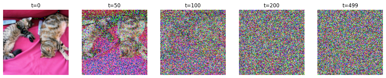
可以使用下面代码可视化一下输出结果：

1
2
3
4
5
6
7
8

for idx, t in enumerate([0, 50, 100, 200, 499]):
    x_noisy = gaussian_diffusion.q_sample(x_start, t=torch.tensor([t]))
    noisy_image = (x_noisy.squeeze().permute(1, 2, 0) + 1) * 127.5
    noisy_image = noisy_image.numpy().astype(np.uint8)
    plt.subplot(1, 5, 1 + idx)
    plt.imshow(noisy_image)
    plt.axis("off")
    plt.title(f"t={t}")

训练目标

训练目标如之前最后所说，就是使用神经网络(第7行的model)去预测之前公式中对图像添加的噪声$\epsilon$,然后目标函数就是最小化模型预测的$\epsilon_\theta(x_t,t)$和$\epsilon$的均方误差。

代码如下：

1
2
3
4
5
6
7
8
9

# compute train losses
def train_losses(self, model, x_start, t):
	# generate random noise
	noise = torch.randn_like(x_start)
	# get x_t
	x_noisy = self.q_sample(x_start, t, noise=noise)
	predicted_noise = model(x_noisy, t)
	loss = F.mse_loss(noise, predicted_noise)
	return loss

训练部分

理解到逆向过程后，接着我们来看一下训练过程，其实就是对于每个batch中的所有图像都需要随机采样一个时间点，用于计算要加的噪声量。

1
2
3
4
5
6
7
8
9
10
11
12
13
14
15
16
17
18
19
20

# train
epochs = 10

for epoch in range(epochs):
    for step, (images, labels) in enumerate(train_loader):
        optimizer.zero_grad()
        
        batch_size = images.shape[0]
        images = images.to(device)
        
        # sample t uniformally for every example in the batch
        t = torch.randint(0, timesteps, (batch_size,), device=device).long()
        
        loss = gaussian_diffusion.train_losses(model, images, t)
        
        if step % 200 == 0:
            print("Loss:", loss.item())
            
        loss.backward()
        optimizer.step()

逆向过程

训练的时候模型学习的是$\epsilon$, 但推理的时候模型需要根据当前的时间步对预测的$\epsilon$做变换得到当前步的预测噪声$\epsilon_t$的$\mu$，从而采样当前步的降噪噪声$\epsilon_t\in\mathcal{N}(\mu,\sigma)$ ($\sigma$已知)

预测当前时间步噪声均值和方差的代码如下所示：

1
2
3
4
5
6
7
8
9
10
11
12
13
14
15
16
17
18
19
20

# Compute the mean and variance of the diffusion posterior: q(x_{t-1} | x_t, x_0)
def q_posterior_mean_variance(self, x_start, x_t, t):
	posterior_mean = (
		self._extract(self.posterior_mean_coef1, t, x_t.shape) * x_start
		+ self._extract(self.posterior_mean_coef2, t, x_t.shape) * x_t
	)
	posterior_variance = self._extract(self.posterior_variance, t, x_t.shape)
	posterior_log_variance_clipped = self._extract(self.posterior_log_variance_clipped, t, x_t.shape)
	return posterior_mean, posterior_variance, posterior_log_variance_clipped
# compute predicted mean and variance of p(x_{t-1} | x_t)
def p_mean_variance(self, model, x_t, t, clip_denoised=True):
	# predict noise using model
	pred_noise = model(x_t, t)
	# get the predicted x_0: different from the algorithm2 in the paper
	x_recon = self.predict_start_from_noise(x_t, t, pred_noise)
	if clip_denoised:
		x_recon = torch.clamp(x_recon, min=-1., max=1.)
	model_mean, posterior_variance, posterior_log_variance = \
				self.q_posterior_mean_variance(x_recon, x_t, t)
	return model_mean, posterior_variance, posterior_log_variance

采样并消除噪声代码如下所示：

第10行中，对数方差乘0.5取指数的含义是，将对数方差转化为方差后开根号得标准差。
公式是：$\sigma = \sqrt{\sigma^2} = \sqrt{e^{\log(\sigma^2)}} = e^{0.5 \cdot \log(\sigma^2)}$

1
2
3
4
5
6
7
8
9
10
11

@torch.no_grad()
def p_sample(self, model, x_t, t, clip_denoised=True):
	# predict mean and variance
	model_mean, _, model_log_variance = self.p_mean_variance(model, x_t, t,
												clip_denoised=clip_denoised)
	noise = torch.randn_like(x_t)
	# no noise when t == 0
	nonzero_mask = ((t != 0).float().view(-1, *([1] * (len(x_t.shape) - 1))))
	# compute x_{t-1}
	pred_img = model_mean + nonzero_mask * (0.5 * model_log_variance).exp() * noise
	return pred_img

推理部分

理解了上面的逆向过程后，推理部分的生成就非常好理解了。就是不断的调用p_sample函数逐渐从一个全噪声生成图像的过程(主函数先调用sample)。

1
2
3
4
5
6
7
8
9
10
11
12
13
14
15
16
17

# denoise: reverse diffusion
@torch.no_grad()
def p_sample_loop(self, model, shape):
	batch_size = shape[0]
	device = next(model.parameters()).device
	# start from pure noise (for each example in the batch)
	img = torch.randn(shape, device=device)
	imgs = []
	for i in tqdm(reversed(range(0, timesteps)), desc='sampling loop time step', total=timesteps):
		img = self.p_sample(model, img, torch.full((batch_size,), i, device=device, dtype=torch.long))
		imgs.append(img.cpu().numpy())
	return imgs

# sample new images
@torch.no_grad()
def sample(self, model, image_size, batch_size=8, channels=3):
	return self.p_sample_loop(model, shape=(batch_size, channels, image_size, image_size))

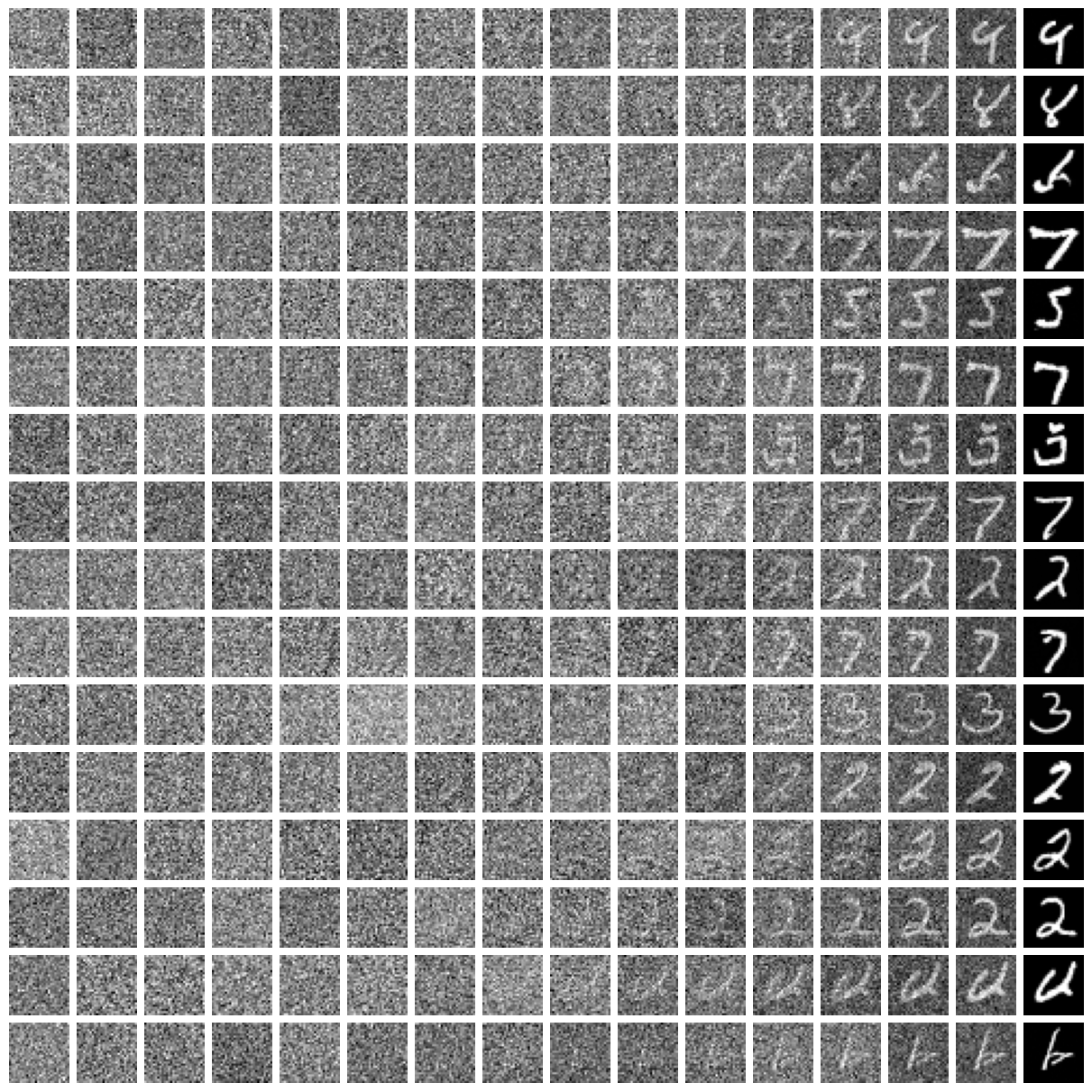
如果要控制diffusion生成特定类别的图像，会使用classifier free guidance方法，后续会讲解。

该ipynb文件最后对于MNIST手写数据集的生成效果如下：