从零开始了解LLaMA：开源大语言模型的架构解析

整理自B站教程：图解llama架构解读源码实现_哔哩哔哩_bilibili

0. 引言

近年来，大型语言模型（LLM）在自然语言处理领域取得了突破性进展，而LLaMA（Large Language Model Meta AI）作为Meta AI开源的一系列LLM，以其优异的性能和开放的姿态，迅速成为研究者和开发者关注的焦点。

你是否好奇LLaMA是如何工作的？它与其他LLM相比有何优势？在这篇博客中，我们将结合代码深入浅出地解析LLaMA的整体架构，带你从零开始了解这一强大的语言模型。我们将探讨LLaMA的模型结构，帮助你全面理解LLaMA的运作机制，并为你开启探索LLM世界的大门。

为了能够更好的配合原代码进行阅读，首先需要安装transformers库：

1	pip install transformers

使用pip show transformers定位到安装包的位置后，使用代码编辑器打开库所在文件夹，我们需要阅读的代码在models/llama文件夹中。

1. 分词器部分

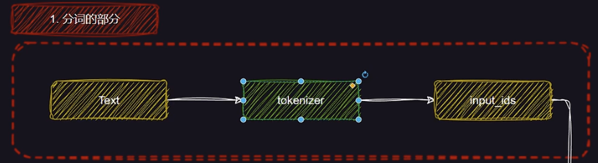
在LLaMA的整体架构中，分词器（Tokenizer）部分负责将原始文本转换为模型能够理解的输入格式。这个过程是深度学习模型处理文本数据的关键步骤，主要通过将文本转换为一系列数字化的ID（即token IDs）来实现。

以一个简单的例子为说明：假设我们有一个文本输入 “I love machine learning.”。分词器首先会将文本分割成以下几个单元：

“I”
“love”
“machine”
“learning”
”.”

接着，分词器将这些词汇映射为对应的数字ID（token IDs）。例如，假设词汇表中的映射为：

“I” -> 101
“love” -> 2057
“machine” -> 12345
“learning” -> 67890
“.” -> 999

最终，分词器输出的token IDs序列为：[101, 2057, 12345, 67890, 999]。这些ID作为LLaMA模型的输入，供模型进行进一步的计算和处理。

通过这种方式，LLaMA能够高效地理解和处理文本数据，为后续的模型计算奠定基础。分词器在这一过程中的作用不仅仅是将文字转为数字，它还要确保分割的单位能够反映出文本的语法和语义结构，从而提高模型的理解能力和生成效果。

2. LLaMA主干部分

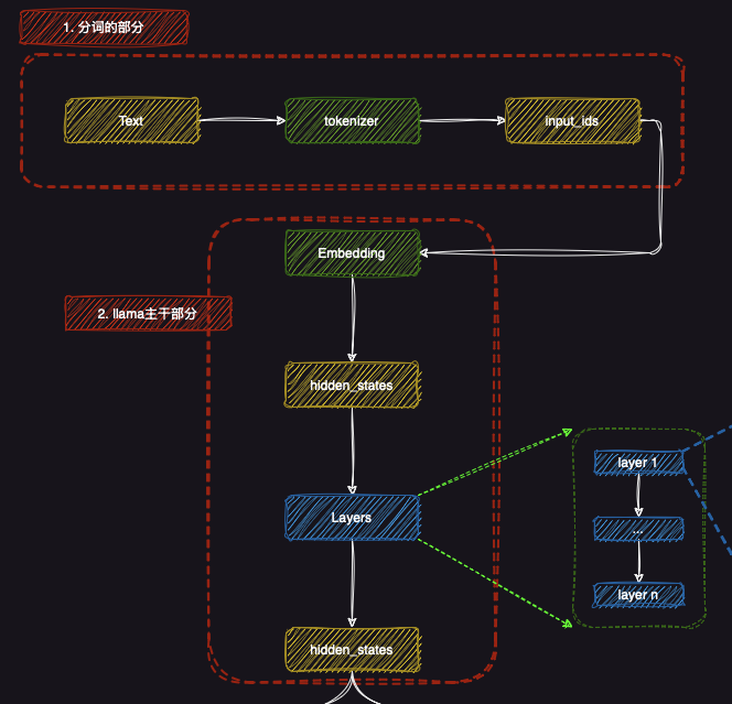
LLaMA的主干部分主要负责对输入文本进行深入的特征提取和理解。这一部分从分词器输出的token IDs开始，经过嵌入层（Embedding），并通过多个隐藏状态（hidden states）层层传递，最终输出模型的高级特征表示。

2.1 嵌入层（Embedding）

在LLaMA模型的主干部分，首先是嵌入层（Embedding）。嵌入层将每个token ID转化为高维向量，使得模型可以在更高层次上理解和处理输入数据。嵌入向量包含了每个token的语义信息，使得模型能够基于这些信息进行后续的计算。

2.2 隐藏状态（hidden states）

从嵌入层输出的向量会进入一系列的隐藏状态（hidden states）。这些隐藏状态是神经网络中每一层的输出，包含了输入数据在网络中的逐步转换过程。LLaMA使用了多个隐藏状态层，这些层共同作用，捕捉了文本中更复杂的语法和语义特征。每一层的输出都会提供关于输入文本的不同方面的理解，帮助模型构建更精确的上下文关系。

2.3 多层处理（Layers）

LLaMA模型的核心部分由多个层（Layers） 组成，每一层都在不断改进模型对输入文本的理解。这些层通过多个神经网络模块，如自注意力机制（Self-attention），帮助模型捕捉长距离依赖关系和复杂的语义信息。每一层都从前一层的输出（即隐藏状态）中提取更高层次的特征表示，逐步增强对文本的理解。在后面我们会结合代码进行具体讲解。

最终，LLaMA通过这些多层的处理机制，能够获得更为丰富的语义表示，进而完成各种语言理解和生成任务。

通过这种结构，LLaMA能够有效地进行文本的深度处理，最大化其对输入的理解能力。每个层级的输出（隐藏状态）都会传递至下一层，以确保模型在每一阶段都能构建出更具语境感知的特征表示。

2.4 代码实现

这一部分的代码对应的就是models/llama/modeling_llama.py中的LlamaModel类

class LlamaModel(LlamaPreTrainedModel):
    """
    Transformer decoder consisting of *config.num_hidden_layers* layers. Each layer is a [`LlamaDecoderLayer`]

    Args:
        config: LlamaConfig
    """

    def __init__(self, config: LlamaConfig):
        super().__init__(config)
        self.padding_idx = config.pad_token_id
        self.vocab_size = config.vocab_size

        self.embed_tokens = nn.Embedding(config.vocab_size, config.hidden_size, self.padding_idx)
        self.layers = nn.ModuleList(
            [LlamaDecoderLayer(config, layer_idx) for layer_idx in range(config.num_hidden_layers)]
        )
        self.norm = LlamaRMSNorm(config.hidden_size, eps=config.rms_norm_eps)
        self.rotary_emb = LlamaRotaryEmbedding(config=config)
        self.gradient_checkpointing = False

        # Initialize weights and apply final processing
        self.post_init()

然后核心的执行顺序如下（forward函数精简版）：

if inputs_embeds is None:
	inputs_embeds = self.embed_tokens(input_ids)

causal_mask = self._update_causal_mask(
		attention_mask, inputs_embeds, cache_position, past_key_values, output_attentions
)

hidden_states = inputs_embeds

# create position embeddings to be shared across the decoder layers
position_embeddings = self.rotary_emb(hidden_states, position_ids)

# hidden states forward(decoder layers)
for decoder_layer in self.layers[: self.config.num_hidden_layers]:
	if output_hidden_states:
		all_hidden_states += (hidden_states,)

	if self.gradient_checkpointing and self.training:
		layer_outputs = self._gradient_checkpointing_func(
			decoder_layer.__call__,
			hidden_states,
			causal_mask,
			position_ids,
			past_key_values,
			output_attentions,
			use_cache,
			cache_position,
			position_embeddings,
		)
	else:
		layer_outputs = decoder_layer(
			hidden_states,
			attention_mask=causal_mask,
			position_ids=position_ids,
			past_key_value=past_key_values,
			output_attentions=output_attentions,
			use_cache=use_cache,
			cache_position=cache_position,
			position_embeddings=position_embeddings,
			**flash_attn_kwargs,
		)

	hidden_states = layer_outputs[0]

	if output_attentions:
		all_self_attns += (layer_outputs[1],)

hidden_states = self.norm(hidden_states)

# add hidden states from the last decoder layer
if output_hidden_states:
	all_hidden_states += (hidden_states,)

output = BaseModelOutputWithPast(
	last_hidden_state=hidden_states,
	past_key_values=past_key_values if use_cache else None,
	hidden_states=all_hidden_states,
	attentions=all_self_attns,
)
return output if return_dict else output.to_tuple()

3. LLaMA的CLM任务

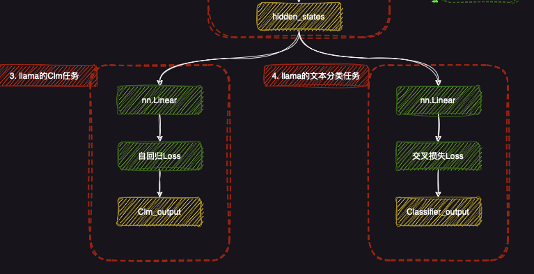
在LLaMA模型中，CLM任务（Causal Language Modeling）是用于训练模型理解文本生成的关键任务之一。其主要目标是通过预测下一个token的方式，训练模型掌握语言的生成能力。

3.1 自回归Loss（Causal Loss）

LLaMA在CLM任务中使用了自回归损失（Causal Loss）。在该任务中，模型基于输入的文本（或token序列）逐步预测每个token，尝试生成下一个token。这一过程通过计算预测值与实际值之间的差距来优化模型，从而使模型能够更准确地预测未来的token。损失函数则根据这个差距来反向传播误差，更新模型参数。

3.2 CLM输出

CLM任务的最终输出是CLM output，即通过训练得到的token预测结果。这个输出包含了每个时间步的预测token，以及其对应的生成概率分布，最终构成了模型的语言生成能力。

3.3 代码实现

这一部分的代码对应的就是models/llama/modeling_llama.py中的LlamaForCausalLM类

class LlamaForCausalLM(LlamaPreTrainedModel, GenerationMixin):
    _tied_weights_keys = ["lm_head.weight"]
    _tp_plan = {"lm_head": "colwise_rep"}

    def __init__(self, config):
        super().__init__(config)
        self.model = LlamaModel(config)
        self.vocab_size = config.vocab_size
        self.lm_head = nn.Linear(config.hidden_size, config.vocab_size, bias=False)

        # Initialize weights and apply final processing
        self.post_init()

可以看到，他上来就定义了一个LlamaModel，利用输出的hidden_states做自回归任务（next token prediction）。

然后我们看forward部分（精简版），输入input_ids，先过上面我们说的model。然后过linear层，最后计算一个loss，loss function的定义见后续代码。

forward部分精简版如下：

# decoder outputs consists of (dec_features, layer_state, dec_hidden, dec_attn)
outputs = self.model(
	input_ids=input_ids,
	attention_mask=attention_mask,
	position_ids=position_ids,
	past_key_values=past_key_values,
	inputs_embeds=inputs_embeds,
	use_cache=use_cache,
	output_attentions=output_attentions,
	output_hidden_states=output_hidden_states,
	return_dict=return_dict,
	cache_position=cache_position,
	**kwargs,
)

hidden_states = outputs[0]
# Only compute necessary logits, and do not upcast them to float if we are not computing the loss
logits = self.lm_head(hidden_states[:, -num_logits_to_keep:, :])

loss = None
if labels is not None:
	loss = self.loss_function(logits=logits, labels=labels, vocab_size=self.config.vocab_size, **kwargs)

if not return_dict:
	output = (logits,) + outputs[1:]
	return (loss,) + output if loss is not None else output

return CausalLMOutputWithPast(
	loss=loss,
	logits=logits,
	past_key_values=outputs.past_key_values,
	hidden_states=outputs.hidden_states,
	attentions=outputs.attentions,
)

loss部分代码如下(默认是ForCausalLM)：

@property
def loss_function(self):
	loss_type = getattr(self, "loss_type", None)

	if loss_type is None or loss_type not in LOSS_MAPPING:
		logger.warning_once(
			f"`loss_type={loss_type}` was set in the config but it is unrecognised."
			f"Using the default loss: `ForCausalLMLoss`."
		)
		loss_type = "ForCausalLM"
	return LOSS_MAPPING[loss_type]

`ForCausalLMLoss` 函数：因果语言模型损失计算

这一部分使用的就是：

def fixed_cross_entropy(source, target, num_items_in_batch: int = None, ignore_index: int = -100, **kwargs):
    reduction = "sum" if num_items_in_batch is not None else "mean"
    loss = nn.functional.cross_entropy(source, target, ignore_index=ignore_index, reduction=reduction)
    if reduction == "sum":
        loss = loss / num_items_in_batch
    return loss

def ForCausalLMLoss(
    logits, labels, vocab_size: int, num_items_in_batch: int = None, ignore_index: int = -100, **kwargs
):
    # Upcast to float if we need to compute the loss to avoid potential precision issues
    logits = logits.float()
    labels = labels.to(logits.device)
    # Shift so that tokens < n predict n
    shift_logits = logits[..., :-1, :].contiguous()
    shift_labels = labels[..., 1:].contiguous()

    # Flatten the tokens
    shift_logits = shift_logits.view(-1, vocab_size)
    shift_labels = shift_labels.view(-1)
    # Enable model parallelism
    shift_labels = shift_labels.to(shift_logits.device)
    loss = fixed_cross_entropy(shift_logits, shift_labels, num_items_in_batch, ignore_index, **kwargs)
    return loss

1. 输入参数

logits: 模型输出，形状 (batch_size, sequence_length, vocab_size)。
labels: 真实标签，形状 (batch_size, sequence_length)。
vocab_size: 词汇表大小。
ignore_index: 忽略的标签索引（如填充符）。

2. 核心步骤

2.1 移位操作

1 2	shift_logits = logits[..., :-1, :] # 预测：去掉最后一个词 shift_labels = labels[..., 1:] # 标签：去掉第一个词

目的: 使模型只能基于前 ( n-1 ) 个词预测第 ( n ) 个词。

2.2 展平

1 2	shift_logits = shift_logits.view(-1, vocab_size) # 展平为 (N, vocab_size) shift_labels = shift_labels.view(-1) # 展平为 (N,)

目的: 将所有预测和标签放在统一维度，方便计算损失。

2.3 计算交叉熵损失

1	loss = fixed_cross_entropy(shift_logits, shift_labels, ...)

公式:
$\text{loss} = -\frac{1}{N} \sum_{i=1}^{N} \sum_{j=1}^{V} y_{ij} \log(p_{ij})$
其中：
- $p_{ij} = \text{softmax}(\text{shift\_logits}_{ij})$ 。
- $y_{ij}$ 是真实标签的 one-hot 编码。

3. 总结

功能: 计算因果语言模型的损失。
核心: 通过移位操作实现因果性，使用交叉熵衡量预测与真实标签的差异。
输出: 损失值（标量）。

示例

输入：

logits: (2, 3, 5)（批次 2，序列 3，词汇表 5）。
labels: (2, 3)。

输出：

shift_logits: (2, 2, 5)。
shift_labels: (2, 2)。
最终损失：标量值。

4. LLaMA的文本分类任务

除了生成任务，LLaMA还支持文本分类任务，这是许多自然语言处理任务的核心部分，特别是在情感分析、主题分类等任务中具有广泛应用。

4.1 分类层（Classifier Layer）

在文本分类任务中，LLaMA通过一个nn.Linear层将隐藏状态（hidden states）转换为适合分类任务的输出。该层根据输入文本的特征，计算出每个类别的概率。

4.2 分类损失（Classification Loss）

LLaMA使用分类损失（Classification Loss） 来优化文本分类任务。与CLM任务不同，分类任务的目标是将文本分配到特定的类别中，损失函数计算预测类别与实际类别之间的差距，并通过反向传播调整模型参数。

4.3 分类输出（Classifier output）

分类任务的输出是Classifier output，即模型对输入文本所预测的分类结果。这个输出表示模型对每个类别的预测概率，并通过选择概率最大的类别作为最终分类结果。

总结来说，LLaMA不仅在语言生成任务（CLM任务）中表现出色，还在文本分类任务中具备强大的能力。通过使用自回归损失和分类损失，LLaMA能够在这两类任务中进行高效的学习与优化，从而实现广泛的自然语言处理应用。

4.4 代码实现

这一部分的代码对应的就是models/llama/modeling_llama.py中的LlamaForSequenceClassification类

class LlamaForSequenceClassification(LlamaPreTrainedModel):
    def __init__(self, config):
        super().__init__(config)
        self.num_labels = config.num_labels
        self.model = LlamaModel(config)
        self.score = nn.Linear(config.hidden_size, self.num_labels, bias=False)

        # Initialize weights and apply final processing
        self.post_init()

然后我们看forward部分（精简版），输入input_ids，先过上面我们说的model。然后过linear层，最后计算一个loss，loss function的定义见后续代码。

forward部分精简版如下：

transformer_outputs = self.model(
	input_ids,
	attention_mask=attention_mask,
	position_ids=position_ids,
	past_key_values=past_key_values,
	inputs_embeds=inputs_embeds,
	use_cache=use_cache,
	output_attentions=output_attentions,
	output_hidden_states=output_hidden_states,
	return_dict=return_dict,
)
hidden_states = transformer_outputs[0]
logits = self.score(hidden_states)

pooled_logits = logits[torch.arange(batch_size, device=logits.device), sequence_lengths]

loss = None
if labels is not None:
	loss = self.loss_function(logits=logits, labels=labels, pooled_logits=pooled_logits, config=self.config)

if not return_dict:
	output = (pooled_logits,) + transformer_outputs[1:]
	return ((loss,) + output) if loss is not None else output

return SequenceClassifierOutputWithPast(
	loss=loss,
	logits=pooled_logits,
	past_key_values=transformer_outputs.past_key_values,
	hidden_states=transformer_outputs.hidden_states,
	attentions=transformer_outputs.attentions,
)

loss还是使用的是交叉熵损失函数，这里不再赘述

然后其实还有两个函数:

4.5 LlamaForQuestionAnswering

任务：问答任务
损失函数：交叉熵损失（Cross-Entropy Loss）
在问答任务中，特别是抽取式问答任务中，LLaMA通常会通过交叉熵损失来计算预测的答案位置与实际答案之间的差距。模型会输出每个token作为答案的概率分布，交叉熵损失用于比较预测的答案跨度与真实答案的跨度之间的差距。
这里的损失函数通常是torch.nn.CrossEntropyLoss，用来对答案span进行评估。

4.6 LlamaForTokenClassification

任务：标记分类任务
损失函数：交叉熵损失（Cross-Entropy Loss）
在标记分类任务中（如命名实体识别、词性标注等），模型会为输入的每个token分配一个标签。每个token的logits将与真实标签进行比较，通常使用交叉熵损失来计算损失。
同样，交叉熵损失通过 torch.nn.CrossEntropyLoss 来实现。

5. LLaMA的Layer层

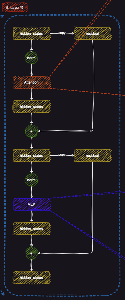
LLaMA的Layer层是模型的核心结构之一，每一层都由多个重要组成部分构成，这些组件共同作用，帮助模型处理输入数据并提取更深层次的特征表示。每一层的处理步骤通常包括自注意力机制（Attention）、归一化（Norm）和多层感知机（MLP）等模块。

5.1 归一化（Norm）

每一层的输入（即隐藏状态hidden states）首先会经过归一化（Norm） 操作。归一化的目的是调整输入的分布，使得模型训练更加稳定，并加速收敛过程。通过这种方式，LLaMA能够确保每一层的输入都处于一个合理的数值范围内。

5.2 自注意力机制（Attention）

接下来，自注意力机制（Attention） 会被应用于每一层的隐藏状态。自注意力机制是LLaMA处理序列数据的关键，它帮助模型根据输入数据的各个部分之间的关系来调整每个token的表示。通过这种方式，模型能够捕捉到序列中远程依赖的关系，从而提升对文本语义的理解能力。注意力机制中的细节会在后面进行详细解释。

在此步骤中，模型会计算每个token与其他token的相关性，并基于这些信息来更新隐藏状态，使得每个token的表示更加贴合上下文。

5.3 残差连接（Residual）

在自注意力模块之后，残差连接（Residual） 被用于将输入隐藏状态与经过自注意力机制更新后的隐藏状态相加，从而形成更新后的隐藏状态。这种残差连接有助于防止梯度消失问题，使得深层模型能够更好地训练。

5.4 多层感知机（MLP）

每一层的后半部分是多层感知机（MLP） 模块，它通常由若干个全连接层（fully connected layers）构成。MLP层的作用是进一步处理更新后的隐藏状态，通过非线性变换来增加模型的表达能力。MLP层帮助模型在处理信息时更好地捕捉复杂的模式。

5.5 残差连接（Residual）

与自注意力机制类似，MLP模块后的输出也会通过一个残差连接与输入进行相加。这样可以确保每一层的特征表示不仅仅依赖于当前层的输出，还结合了输入的信息，使得梯度能够顺利传播，从而提高训练效果。

5.6 最终输出（hidden states）

经过上述步骤，每一层的最终输出是更新后的隐藏状态（hidden states），它包含了模型在该层提取到的所有语义信息。这些隐藏状态将被传递到下一层，继续进行进一步的处理，直到整个网络完成训练。

总结来说，LLaMA的每一层通过自注意力、归一化、MLP和残差连接等模块的协作，能够从输入数据中提取越来越丰富的特征。这些层级的组合构建了一个深度神经网络，使得LLaMA能够在多个自然语言处理任务中取得良好的效果。

5.7 代码实现

这一部分的代码对应的就是models/llama/modeling_llama.py中的LlamaDecoderLayer类

class LlamaDecoderLayer(nn.Module):
    def __init__(self, config: LlamaConfig, layer_idx: int):
        super().__init__()
        self.hidden_size = config.hidden_size

        self.self_attn = LlamaAttention(config=config, layer_idx=layer_idx)

        self.mlp = LlamaMLP(config)
        self.input_layernorm = LlamaRMSNorm(config.hidden_size, eps=config.rms_norm_eps)
        self.post_attention_layernorm = LlamaRMSNorm(config.hidden_size, eps=config.rms_norm_eps)

可以看到确实如我们之前所介绍那样，包含了3个部分：

Attention部分
MLP部分
标准化部分

forward函数实现如下：

residual = hidden_states

hidden_states = self.input_layernorm(hidden_states)

# Self Attention
hidden_states, self_attn_weights = self.self_attn(
	hidden_states=hidden_states,
	attention_mask=attention_mask,
	position_ids=position_ids,
	past_key_value=past_key_value,
	output_attentions=output_attentions,
	use_cache=use_cache,
	cache_position=cache_position,
	position_embeddings=position_embeddings,
	**kwargs,
)
hidden_states = residual + hidden_states

# Fully Connected
residual = hidden_states
hidden_states = self.post_attention_layernorm(hidden_states)
hidden_states = self.mlp(hidden_states)
hidden_states = residual + hidden_states

outputs = (hidden_states,)
if output_attentions:
	outputs += (self_attn_weights,)

return outputs

可以看到就是如上图所示的一个流程。

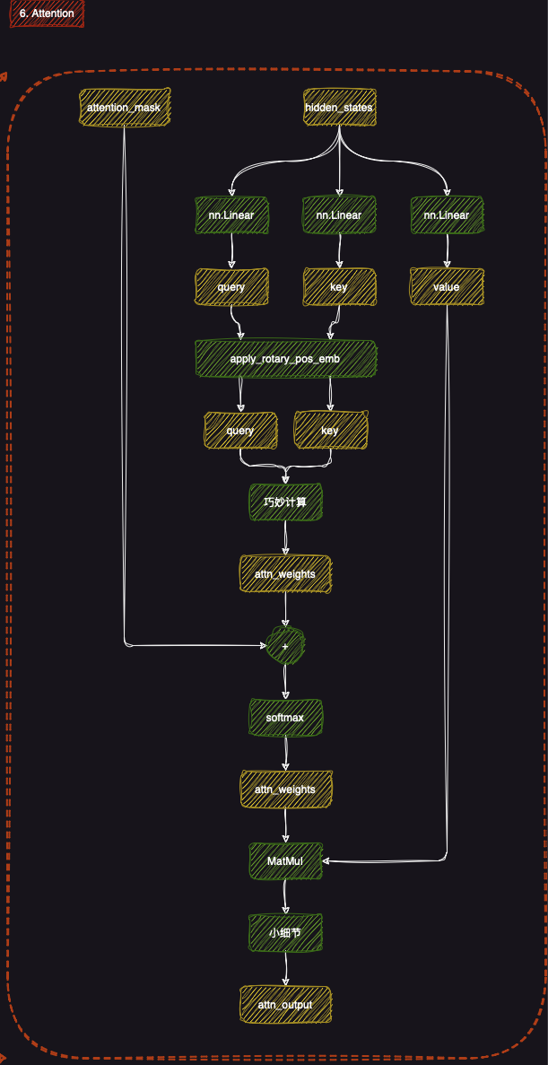
6. Attention部分

在LLaMA模型中，Attention机制是一个关键的模块，帮助模型在处理文本时捕捉不同位置之间的依赖关系。通过这种机制，模型能够动态地关注输入序列中与当前token相关的部分，从而改善对上下文的理解。

6.1 输入处理

首先，模型会将隐藏状态（hidden states）通过线性层（nn.Linear）转换为查询（query） 、键（key）和值（value）。这些表示将作为自注意力计算的核心输入。

6.2 旋转位置编码（apply_rotary_pos_emb）

接着，通过旋转位置编码（apply_rotary_pos_emb） 对查询和键进行位置编码。这一步确保模型能够捕捉到输入中各token的位置信息，从而正确理解其在上下文中的角色。

6.3 计算注意力权重

然后，查询和键将进行点积计算，并通过softmax函数得到注意力权重（attn_weights）。这些权重表示每个token在当前上下文中对其他token的“关注程度”。

6.4 计算输出

最后，注意力权重会与值（value）进行矩阵乘法（MatMul），从而得到最终的Attention输出（attn_output）。这个输出表示了模型基于输入文本中各部分关系所做的加权汇总。

6.5 代码实现

这一部分的代码对应的就是models/llama/modeling_llama.py中的LlamaAttention类

class LlamaAttention(nn.Module):
    """Multi-headed attention from 'Attention Is All You Need' paper"""

    def __init__(self, config: LlamaConfig, layer_idx: int):
        super().__init__()
        self.config = config
        self.layer_idx = layer_idx
        self.head_dim = getattr(config, "head_dim", config.hidden_size // config.num_attention_heads)
        self.num_key_value_groups = config.num_attention_heads // config.num_key_value_heads
        self.scaling = self.head_dim**-0.5
        self.attention_dropout = config.attention_dropout
        self.is_causal = True

        self.q_proj = nn.Linear(
            config.hidden_size, config.num_attention_heads * self.head_dim, bias=config.attention_bias
        )
        self.k_proj = nn.Linear(
            config.hidden_size, config.num_key_value_heads * self.head_dim, bias=config.attention_bias
        )
        self.v_proj = nn.Linear(
            config.hidden_size, config.num_key_value_heads * self.head_dim, bias=config.attention_bias
        )
        self.o_proj = nn.Linear(
            config.num_attention_heads * self.head_dim, config.hidden_size, bias=config.attention_bias
        )

forward函数实现如下（精简版）：

input_shape = hidden_states.shape[:-1]
hidden_shape = (*input_shape, -1, self.head_dim)

query_states = self.q_proj(hidden_states).view(hidden_shape).transpose(1, 2)
key_states = self.k_proj(hidden_states).view(hidden_shape).transpose(1, 2)
value_states = self.v_proj(hidden_states).view(hidden_shape).transpose(1, 2)

cos, sin = position_embeddings
query_states, key_states = apply_rotary_pos_emb(query_states, key_states, cos, sin)

if past_key_value is not None:
	# sin and cos are specific to RoPE models; cache_position needed for the static cache
	cache_kwargs = {"sin": sin, "cos": cos, "cache_position": cache_position}
	key_states, value_states = past_key_value.update(key_states, value_states, self.layer_idx, cache_kwargs)
attn_output, attn_weights = attention_interface(
	self,
	query_states,
	key_states,
	value_states,
	attention_mask,
	dropout=0.0 if not self.training else self.attention_dropout,
	scaling=self.scaling,
	**kwargs,
)

attn_output = attn_output.reshape(*input_shape, -1).contiguous()
attn_output = self.o_proj(attn_output)
return attn_output, attn_weights

对于Attention中的一些重要技术如RoPE以及Paged Attention等后续会单开栏目进行介绍。

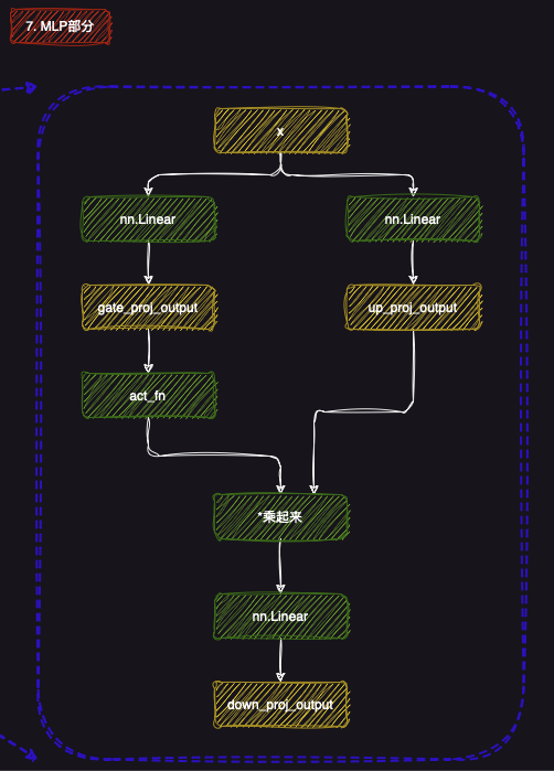
7. MLP部分

7.1 简介

MLP这一部分的设计则更为简单，详细设计后续会结合代码进行进一步的讲解，简单介绍下为什么这样设计：

门控与投影的结合：通过将gate_proj_output和up_proj_output相乘，模型能够在每一层中灵活地调整信息流动。这种设计通过加权和门控的方式，确保模型能够有选择性地保留或抑制不同的输入特征，从而提高处理能力。（up是升采样的流程，down是降采样的过程）
非线性激活：激活函数的引入确保了模型能够捕捉复杂的非线性模式，使得LLaMA可以更好地拟合数据中的复杂关系，提升模型的准确性和泛化能力。

7.2 代码实现

这一部分的代码对应的就是models/llama/modeling_llama.py中的LlamaMLP类

代码如下：

class LlamaMLP(nn.Module):
    def __init__(self, config):
        super().__init__()
        self.config = config
        self.hidden_size = config.hidden_size
        self.intermediate_size = config.intermediate_size
        self.gate_proj = nn.Linear(self.hidden_size, self.intermediate_size, bias=config.mlp_bias)
        self.up_proj = nn.Linear(self.hidden_size, self.intermediate_size, bias=config.mlp_bias)
        self.down_proj = nn.Linear(self.intermediate_size, self.hidden_size, bias=config.mlp_bias)
        self.act_fn = ACT2FN[config.hidden_act]

    def forward(self, x):
        down_proj = self.down_proj(self.act_fn(self.gate_proj(x)) * self.up_proj(x))
        return down_proj

其中self.act_fn指的是激活函数，符合上图所示的运算步骤

8. 归一化部分（RMSNorm）

8.1 简介

在LLaMA模型中，RMSNorm（均方根归一化）是一种用于归一化的技术，类似于传统的Layer Normalization，但采用了不同的归一化方式。与LayerNorm基于均值和方差的标准化不同，RMSNorm只使用输入的方差（而非均值），通过计算均方根（RMS）来调整每个token的特征。这种方法的优势在于数值计算的简化与稳定性，尤其是在处理大规模预训练模型时。RMSNorm能够避免训练过程中出现的梯度消失或爆炸问题，并在许多任务中展现了出色的性能。

与标准化方法（如LayerNorm）不同，RMSNorm不需要中心化输入数据，而是直接对每个token的特征进行归一化，保留了输入数据的原始分布。这使得它在大规模神经网络训练中具有更高的效率与稳定性，尤其适用于像LLaMA这样的大型模型。

接下来，我们将深入探讨 LlamaRMSNorm 层的实现和工作原理。

8.2 代码实现

这一部分的代码对应的就是models/llama/modeling_llama.py中的LlamaMLP类

class LlamaRMSNorm(nn.Module):
    def __init__(self, hidden_size, eps=1e-6):
        """
        LlamaRMSNorm is equivalent to T5LayerNorm
        """
        super().__init__()
        self.weight = nn.Parameter(torch.ones(hidden_size))
        self.variance_epsilon = eps

    def forward(self, hidden_states):
        input_dtype = hidden_states.dtype
        hidden_states = hidden_states.to(torch.float32)
        variance = hidden_states.pow(2).mean(-1, keepdim=True)
        hidden_states = hidden_states * torch.rsqrt(variance + self.variance_epsilon)
        return self.weight * hidden_states.to(input_dtype)

    def extra_repr(self):
        return f"{tuple(self.weight.shape)}, eps={self.variance_epsilon}"

LlamaRMSNorm 是一种归一化方法，类似于 T5 模型中的 T5LayerNorm，但它使用 均方根（RMS）归一化，而不是常规的标准化方法（如 LayerNorm）。这种方法通过对输入的方差进行归一化，使得模型在训练时更加稳定。

数学公式

均方根归一化的核心公式如下：

\hat{x}_i = \frac{x_i}{\sqrt{\frac{1}{N} \sum_{i=1}^N x_i^2 + \epsilon}}

其中：

$x_i$ 是输入的第 $i$ 个元素（例如某个token的特征值）。
$N$ 是特征维度的大小。
$\epsilon$ 是防止除零错误的小常数（例如 $1e-6$ ）。
$\hat{x}_i$ 是归一化后的输出。

1. 初始化

1 2	self.weight = nn.Parameter(torch.ones(hidden_size)) self.variance_epsilon = eps

self.weight：一个可学习的参数，用于对归一化后的隐藏状态进行缩放，初始值为 1。
self.variance_epsilon：小常数 eps，用于防止除零错误。

2. 前向传播

hidden_states = hidden_states.to(torch.float32)
variance = hidden_states.pow(2).mean(-1, keepdim=True)
hidden_states = hidden_states * torch.rsqrt(variance + self.variance_epsilon)
return self.weight * hidden_states.to(input_dtype)

计算方差：首先将输入 hidden_states 转换为 float32，然后沿特征维度计算方差。
均方根归一化：使用 torch.rsqrt() 对方差加上小常数 eps 后取平方根的倒数，进行归一化处理。
缩放和恢复数据类型：归一化后的结果乘以可学习的 weight 参数，并恢复到输入的原始数据类型。

3. 额外显示信息

1 2	def extra_repr(self): return f"{tuple(self.weight.shape)}, eps={self.variance_epsilon}"

extra_repr() 用于返回该层的额外信息，便于调试。

总结

LlamaRMSNorm 是一种优化的归一化方法，常用于 LLaMA 模型。它通过计算输入的方差并对其进行均方根归一化，使用可学习的参数进行缩放，帮助模型在训练过程中保持稳定性。与传统的标准化方法相比，RMSNorm 在一些任务中表现出更好的效果，尤其是在处理大规模模型时。

9. 代码调试深入理解

为了能够更深入的理解Llama，可以对下面的代码进行调试，一步一步调试进去就可以对Llama3模型的架构掌握的更加清晰：

from transformers.models.llama import LlamaModel, LlamaConfig
import torch

def run_llama():
    # 1. 模型初始化
    llamaconfig = LlamaConfig(vocab_size=32000, hidden_size=4096//2,
                              intermediate_size=11000//2,
                              num_hidden_layers=32//2,
                              num_attention_heads=32//2,
                              max_position_embeddings=2048//2)
    llamamodel = LlamaModel(config=llamaconfig)
    # 2. 定义输入 batchsize=4
    inputs_ids = torch.randint(
        low=0, high=llamaconfig.vocab_size, size=(4, 30))
    # 3. 进行推理forward
    res = llamamodel(inputs_ids)
    print(res)
    
if __name__ == '__main__':
    run_llama()

在这段代码中，我们使用 Hugging Face 的 transformers 库来初始化和运行一个简化版的 LLaMA 模型。LLaMA 是一种基于 Transformer 架构的大语言模型，广泛应用于自然语言处理任务。代码首先通过 LlamaConfig 定义了模型的配置参数，如词汇表大小、隐藏层维度、注意力头数等，并将原始模型的参数减半以降低计算成本。接着，我们生成了一个随机的输入张量，形状为 (4, 30)，表示 4 个样本，每个样本长度为 30。最后，将输入传递给模型进行推理，并输出结果。这段代码展示了如何快速搭建和运行一个简化版的 LLaMA 模型，适合初学者了解模型的基本使用流程。

根据代码调试，不难知道，针对上面这个代码，hidden_states的大小为[4, 30, 2048]因为中间是transformer结构，所以hidden_states的大小不会发生变化（多头注意力的时候是先proj再分多头）

更完整的一个推理过程调试可以采用下面这个代码：

from transformers import AutoTokenizer, LlamaForCausalLM
import torch

# 指定模型路径
model_path = "/home/vegetabot/Filesys/CodeField_win/LLaMA-Factory/Meta-Llama-3-8B-Instruct"

# ✅ 使用 AutoTokenizer，让它自动匹配 Llama 3 的 tokenizer
tokenizer = AutoTokenizer.from_pretrained(model_path, legacy=False)

# ✅ 直接使用 LlamaForCausalLM
model = LlamaForCausalLM.from_pretrained(model_path, torch_dtype=torch.bfloat16).to("cuda")

# 预编译模型，加速推理
model = torch.compile(model)
print("✅ Model Compilation Complete!")

# 输入文本
# input_text = "你好，请问 Llama 3 有哪些新特性？请使用中文回答"
input_text = "你好，请问Llama 3 有哪些新特性？请使用中文回答"

# 编码输入文本
inputs = tokenizer(input_text, return_tensors="pt").to("cuda")

# 生成文本（使用 KV Cache 加速）
outputs = model.generate(**inputs, max_new_tokens=1000, use_cache=True)

# 解码输出
generated_text = tokenizer.decode(outputs[0], skip_special_tokens=True)
print("🤖 Llama 3 生成的回答：\n", generated_text)

在这段优化后的代码中，我们使用 Hugging Face 的 transformers 库快速调用 Meta-Llama-3-8B-Instruct 模型进行中文对话生成。首先通过 AutoTokenizer 和 AutoModelForCausalLM 加载本地预训练的分词器和模型（需提前下载模型权重），并以 bfloat16 精度量化模型以降低显存占用。接着利用 torch.compile 对模型进行编译优化，加速推理效率。输入问题 “你好，请问 Llama 3 有哪些新特性？” 被编码为 GPU 张量后，模型通过 generate 方法生成最多 1000 个新 token 的回答，最终解码输出自然流畅的中文文本。整个过程展示了如何高效部署大语言模型并进行交互式推理。

经过调试，不难知道，输入的query首先经过tokenizer被编码成了[1,20]大小的向量。然后再进模型进行推理，其中hidden_states的大小为[1,20,4096],使用的attention是sdp attention，然后我们的RoPE作用在Q K上，注意力机制的头数为32。

对于MLP层，隐藏层是从4096先变化到14336然后再被映射回来，采用的激活函数是SiLU。一共是有32层Decoder Layer

过对LLaMA架构的深入解析，我们可以看到，它的设计巧妙地平衡了性能与效率，为自然语言处理领域提供了强大的工具。无论是研究者还是开发者，LLaMA的开源都为我们探索语言模型的潜力打开了新的大门。希望这篇博客能帮助你更好地理解LLaMA，也希望它能激发你对大语言模型的更多兴趣与思考。未来已来，让我们一起期待更多创新与突破！

本文采用署名-非商业性使用-相同方式共享 4.0 国际许可协议，转载请注明出处。

从零开始了解LLaMA：开源大语言模型的架构解析

0. 引言

1. 分词器部分

2. LLaMA主干部分

2.1 嵌入层（Embedding）

2.2 隐藏状态（hidden states）

2.3 多层处理（Layers）

2.4 代码实现

3. LLaMA的CLM任务

3.1 自回归Loss（Causal Loss）

3.2 CLM输出

3.3 代码实现

ForCausalLMLoss 函数：因果语言模型损失计算

1. 输入参数

2. 核心步骤

3. 总结

示例

4. LLaMA的文本分类任务

4.1 分类层（Classifier Layer）

4.2 分类损失（Classification Loss）

4.3 分类输出（Classifier output）

4.4 代码实现

4.5 LlamaForQuestionAnswering

4.6 LlamaForTokenClassification

5. LLaMA的Layer层

5.1 归一化（Norm）

5.2 自注意力机制（Attention）

5.3 残差连接（Residual）

5.4 多层感知机（MLP）

5.5 残差连接（Residual）

5.6 最终输出（hidden states）

5.7 代码实现

6. Attention部分

6.1 输入处理

6.2 旋转位置编码（apply_rotary_pos_emb）

6.3 计算注意力权重

6.4 计算输出

6.5 代码实现

7. MLP部分

7.1 简介

7.2 代码实现

8. 归一化部分（RMSNorm）

8.1 简介

8.2 代码实现

数学公式

1. 初始化

2. 前向传播

3. 额外显示信息

总结

9. 代码调试深入理解

`ForCausalLMLoss` 函数：因果语言模型损失计算