PyTorch：PyTorch RNN&LSTM

序列表示（Sequence representation）

方法一

对于一个句子，我们采用如下的表示方式：

[seq\_len,feature\_len]

$seq \_ len$ 表示的是这个句子所含的单词数量， $feature \_ len$ 表示的是表示一个单词所需向量的长度（一般采用独热编码）。

缺点：独热码使得矩阵变得稀疏，占用了大量存储空间的同时，表达的信息海非常少，这不是我们想看到的结果。

方法二

为了让特征向量变得不那么稀疏，我们不采用独热编码方式。我们还是可以将要使用的单词使用向量编码，只不过这次向量编码有效的利用了语义相关性，语义相关性高的两个向量，他们的夹角更小，反之，夹角会非常大。现目前已经有两种技术我们可以使用来进行这种方式的编码。

Word2vec
GloVe

因为不会深入nlp部分，所以我们暂时不详细介绍这两种方式，大家有兴趣可以自行百度。

方法二也是现目前使用最广泛的一种方法。

PyTorch实现

使用PyTorch 建立索引特征向量表并根据索引查询对应单词的特征向量

import torch
from torch import nn

word_to_ix={"hello": 0,"world" :1}

lookup_tensor  = torch.tensor([word_to_ix["hello"]],dtype=torch.long)

embeds=nn.Embedding(2,5)
hello_embed=embeds(lookup_tensor)
print(hello_embed)

运行结果

1 2	tensor([[-0.4940, -0.9166, 1.2154, 0.4011, -0.6101]], grad_fn=<EmbeddingBackward0>)

PyTorch 导入GloVe

GloVe是一种nlp中常用的单词的向量编码。

在PyTorch中使用GloVe编码的代码如下：

from torchnlp.word_to_vector import GloVe
vectors=GloVe()

print(vectors['hello']) # 然后就可以得到向量表示的结果

RNN原理

所具备的能力

能处理长句子，普通的全连接神经网络不行，因为这样w,b参数太多了。解决方式是采用了权值共享
能够连接上下文，具有上下文语境信息（语境贯穿）

RNN原理图

具体一般情况下的表达式如下：

h_t=f_w(h_{t-1},x_t)

h_t=tanh(W_{hh}h_{t-1}+W_{xh}x_t)\qquad(there\ are \ two \ bias!)

y_t=W_{hy}h_t

反向传播更新梯度的公式

\frac{\partial E_t}{\partial W_{hh}}=\sum_{i=0}^t \frac{\partial E_t}{\partial y_t}\frac{\partial y_t}{\partial h_t}\frac{\partial h_t}{\partial h_i}\frac{\partial h_i}{\partial W_{hh}}

如果我们采用 $[seq\_len,batch\_sz,feature\_len]$ 来表示数据，则对于数据大小为[5,3,100]的语义数据来说，我们输入RNN中 $x_i$ 的维度应该是[3,100]也就是 $[batch\_sz,feature\_len]$

RNN Layer使用

请牢记

x_t@w_{xh}+h_t@w_{hh}

`nn.RNN`

首先举一个简单的例子让我们来看一看该API中的参数信息

In [3]: from torch import nn
In [4]: rnn=nn.RNN(100,20)
In [5]: rnn._parameters.keys()
Out[5]: odict_keys(['weight_ih_l0', 'weight_hh_l0', 'bias_ih_l0', 'bias_hh_l0'])
In [6]: rnn.weight_hh_l0.shape,rnn.weight_ih_l0.shape
Out[6]: (torch.Size([20, 20]), torch.Size([20, 100]))
In [7]: rnn.bias_hh_l0.shape,rnn.bias_ih_l0.shape
Out[7]: (torch.Size([20]), torch.Size([20]))

一般来说该API填入参数是`nn.RNN(input_size,hidden_size,byn_layers)`

input_size:代表的是表示一个单词所需的向量的长度。 hidden_size:代表的是输出的时候向量的长度。 byn_layers:代表的是输入到输出中间层的个数，默认层数为一层

因为上面代码没写`byn_layers`参数

，所以默认一层，因此上面的网络参数结尾数字都是0。

forward

1	out,ht=forward(x,h0)

x：网络输入，tensor大小为 $[seq\_len,batchsz,word\_vec]$

h0：RNN的初始输入，tensor大小为 $[num\_layers,batchsz,h\_dim]$ 其实可以不写，forword对于一个长度为seq_len的句子，会将循环神经网络全部执行一遍（每个单词按顺序一次扔进去更新模型参数）。

ht：tensor大小为 $[num\_layers,batchsz,h\_dim]$ ,表示的是最后一个单词送入后，最后一个MLP的每一层的输出

out：tensor大小为 $[seq\_len,batchsz,h\_dim]$ ,表示的是每送入一个单词后，每一个MLP的最后一层的输出

h_dim就是上面的hidden_size

下面举一个例子更加具体的来说明这个API的使用方法。

这是一个单层的RNN

In [3]: from torch import nn
In [4]: rnn=nn.RNN(input_size=100, hidden_size=20,num_layers=1)
In [5]: print(rnn)
RNN(100, 20)
In [6]: x=torch.randn(10,3,100)
In [7]: out,ht=rnn(x,torch.zeros(1,3,20))
In [8]: print(out.shape)
torch.Size([10, 3, 20])

仔细阅读代码会发现和前面说的一样，很好的验证了前面我们说的正确性。

多层RNN

原理一样，这里放个代码来观察一下PyTorch中RNN模块的参数定义和多层RNN设计规则。

In [3]: from torch import nn
In [4]: rnn=nn.RNN(100,10,num_layers=2)
In [5]: rnn._parameters.keys()
Out[5]: odict_keys(['weight_ih_l0', 'weight_hh_l0', 'bias_ih_l0', 'bias_hh_l0', 'weight_ih_l1', 'weight_hh_l1', 'bias_ih_l1', 'bias_hh_l1'])
In [6]: rnn.weight_hh_l0.shape, rnn.weight_ih_l0.shape
Out[6]: (torch.Size([10, 10]), torch.Size([10, 100]))
In [7]: rnn.weight_hh_l1.shape, rnn.weight_ih_l1.shape
Out[7]: (torch.Size([10, 10]), torch.Size([10, 10]))

注意观察rnn.weight_ih_l0.shape和rnn.weight_ih_l1.shape的维度区别

同理我们也给出和上面单层比较像的4层RNN代码，帮助大家理解。

In [3]: from torch import nn
In [4]: rnn=nn.RNN(input_size=100,hidden_size=20,num_layers=4)
In [5]: print(rnn)
RNN(100, 20, num_layers=4)
In [6]: x=torch.randn(10,3,100)
In [7]: out,h=rnn(x)
In [8]: print(out.shape,h.shape)
torch.Size([10, 3, 20]) torch.Size([4, 3, 20])

`nn.RNNCell`

不同于nn.RNN,该函数需要我们多次input才能迭代出最后的结果。打比方就是比如说我有一句话，其中有10个单词。对于nn.RNN我们只需要一起input进去，nn.RNN迭代一次就自动更新了所有，而nn.RNNCell我们要按顺序一个单词一个单词扔进去训练。相比之下nn.RNNCell虽然更加麻烦，但是比nn.RNN更加灵活。

初始化

1	rnncell=nn.RNNCell(100,20)

两个参数表示输入和输出的维度，感觉和nn.Linear有点像

使用方法

1	ht=rnncell(xt,ht_1)

xt：当前网络输入，tensor大小为 $[batchsz,word\_vec]$

ht_1：上一次RNN输出，tensor大小为 $[num\_layers,batchsz,h\_dim]$ ，和之前那一样

ht：本次RNN输出，tensor大小为 $[num\_layers,batchsz,h\_dim]$

迭代操作

单层RNN

In [3]: from torch import nn
In [4]: cell1=nn.RNNCell(100,20)
In [5]: h1=torch.zeros(3,20)
In [6]: for xt in x:
   ...:     h1=cell1(xt,h1)
In [7]: print(h1.shape)
torch.Size([3,20])

双层RNN

In [3]: from torch import nn
In [4]: cell1=nn.RNNCell(100,30)
In [5]: h1=torch.zeros(3,30)
In [6]: cell2=nn.RNNCell(30,20)
In [7]: h2=torch.zeros(3,20)
In [8]: for xt in x:
   ...:     h1=cell1(xt,h1)
   ...:     h2=cell2(h1,h2)
In [9]: print(h2.shape)
torch.Size([3,20])

实战RNN波形预测

这里想实现的一个目的就是根据正弦波形的前段部分，预测后面的正弦曲线走势。

正弦曲线预测

我们这里实现的功能是根据前1个值预测后1个值是多少。

训练是每次扔入连续的50个值，然后预测向后预测仅往后移动一个单位的50个值（有49个值是重复的）

网络设计

class Net(nn.Module):

    def __init__(self, ):
        super(Net, self).__init__()

        self.rnn = nn.RNN(
            input_size=input_size,
            hidden_size=hidden_size,
            num_layers=1,
            batch_first=True, #input:[b,seq_len,word_vec]
        )
        # 初始化参数
        for p in self.rnn.parameters():
          nn.init.normal_(p, mean=0.0, std=0.001)

        self.linear = nn.Linear(hidden_size, output_size)

    def forward(self, x, hidden_prev):

       out, hidden_prev = self.rnn(x, hidden_prev)
       # [b, seq, h]
       out = out.view(-1, hidden_size)
       out = self.linear(out)
       out = out.unsqueeze(dim=0)
       return out, hidden_prev

训练部分

for iter in range(6000):
    start = np.random.randint(3, size=1)[0]
    time_steps = np.linspace(start, start + 10, num_time_steps)
    data = np.sin(time_steps)
    data = data.reshape(num_time_steps, 1)
    x = torch.tensor(data[:-1]).float().view(1, num_time_steps - 1, 1)
    y = torch.tensor(data[1:]).float().view(1, num_time_steps - 1, 1)

    output, hidden_prev = model(x, hidden_prev)
    hidden_prev = hidden_prev.detach()

    loss = criterion(output, y)
    model.zero_grad()
    loss.backward()
    # for p in model.parameters():
    #     print(p.grad.norm())
    # torch.nn.utils.clip_grad_norm_(p, 10)
    optimizer.step()

    if iter % 100 == 0:
        print("Iteration: {} loss {}".format(iter, loss.item()))

代码中的detach是我们之前从未见过的函数。它返回一个新的tensor，从当前计算图中分离下来。但是仍指向原变量的存放位置，**不同之处只是requirse_grad为false.**得到的这个tensir永远不需要计算器梯度，不具有grad.

测试部分

start = np.random.randint(3, size=1)[0]
time_steps = np.linspace(start, start + 10, num_time_steps)
data = np.sin(time_steps)
data = data.reshape(num_time_steps, 1)
x = torch.tensor(data[:-1]).float().view(1, num_time_steps - 1, 1)
y = torch.tensor(data[1:]).float().view(1, num_time_steps - 1, 1)

predictions = []
input = x[:, 0, :]
for _ in range(x.shape[1]):
  input = input.view(1, 1, 1)
  (pred, hidden_prev) = model(input, hidden_prev)
  input = pred
  predictions.append(pred.detach().numpy().ravel()[0])

x = x.data.numpy().ravel()
y = y.data.numpy()
plt.scatter(time_steps[:-1], x.ravel(), s=90)
plt.plot(time_steps[:-1], x.ravel())

plt.scatter(time_steps[1:], predictions)
plt.show()

代码汇总

import  numpy as np
import  torch
import  torch.nn as nn
import  torch.optim as optim
from    matplotlib import pyplot as plt


num_time_steps = 50
input_size = 1
hidden_size = 16
output_size = 1
lr=0.01



class Net(nn.Module):

    def __init__(self, ):
        super(Net, self).__init__()

        self.rnn = nn.RNN(
            input_size=input_size,
            hidden_size=hidden_size,
            num_layers=1,
            batch_first=True,
        )
        for p in self.rnn.parameters():
          nn.init.normal_(p, mean=0.0, std=0.001)

        self.linear = nn.Linear(hidden_size, output_size)

    def forward(self, x, hidden_prev):

       out, hidden_prev = self.rnn(x, hidden_prev)
       # [b, seq, h]
       out = out.view(-1, hidden_size)
       out = self.linear(out)
       out = out.unsqueeze(dim=0)
       return out, hidden_prev




model = Net()
criterion = nn.MSELoss()
optimizer = optim.Adam(model.parameters(), lr)

hidden_prev = torch.zeros(1, 1, hidden_size)

for iter in range(6000):
    start = np.random.randint(3, size=1)[0]
    time_steps = np.linspace(start, start + 10, num_time_steps)
    data = np.sin(time_steps)
    data = data.reshape(num_time_steps, 1)
    x = torch.tensor(data[:-1]).float().view(1, num_time_steps - 1, 1)
    y = torch.tensor(data[1:]).float().view(1, num_time_steps - 1, 1)

    output, hidden_prev = model(x, hidden_prev)
    hidden_prev = hidden_prev.detach()

    loss = criterion(output, y)
    model.zero_grad()
    loss.backward()
    # for p in model.parameters():
    #     print(p.grad.norm())
    # torch.nn.utils.clip_grad_norm_(p, 10)
    optimizer.step()

    if iter % 100 == 0:
        print("Iteration: {} loss {}".format(iter, loss.item()))

start = np.random.randint(3, size=1)[0]
time_steps = np.linspace(start, start + 10, num_time_steps)
data = np.sin(time_steps)
data = data.reshape(num_time_steps, 1)
x = torch.tensor(data[:-1]).float().view(1, num_time_steps - 1, 1)
y = torch.tensor(data[1:]).float().view(1, num_time_steps - 1, 1)

predictions = []
input = x[:, 0, :]
for _ in range(x.shape[1]):
  input = input.view(1, 1, 1)
  (pred, hidden_prev) = model(input, hidden_prev)
  input = pred
  predictions.append(pred.detach().numpy().ravel()[0])

x = x.data.numpy().ravel()
y = y.data.numpy()
plt.scatter(time_steps[:-1], x.ravel(), s=90)
plt.plot(time_steps[:-1], x.ravel())

plt.scatter(time_steps[1:], predictions)
plt.show()

ravel()在numpy中是将numpy数组拍平，变成一维的操作，类似前面讲的Flatten

结果

预测结果（橙色点）

RNN训练问题

梯度爆炸
梯度弥散

梯度爆炸

梯度爆炸示意图

解决方法

其实并不是很难，我们采用clipping的方法，就是我们每次使用backward()更新了梯度信息后，对所得到的梯度大小进行判断，如果模长大于了阈值，则我们对该梯度( $\vec{grad}$ )进行如下操作:

\vec{grad}=threshold\times \frac{\vec{grad}}{||grad||}

虽然没有从根本解决梯度爆炸的问题，但是我们有效遏制了它带来的糟糕的情况。

有clipping和无clipping情况的对比

注意是对参数的梯度进行clipping不是对网络中的参数本体！！！

PyTorch实现

所使用的函数是torch.nn.utils.clip_grad_norm_

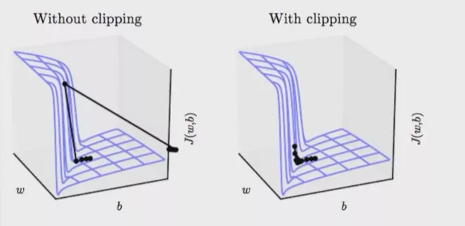
loss = criterion(output,y)
model.zero_grad()
loss.backward()
for p in model.parameters():
	print(p.grad.norm())
	torch.nn.utils.clip_grad_norm_(p,10) # <10
optimizer.step()

梯度在10左右比较合适

梯度弥散

RNN梯度弥散的解决方法，请见下节课所讲的LSTM

LSTM

大体结构和RNN相同只是多了三个 $\sigma$ (sigmoid)函数来作为门，这三道门分别叫做Forget gate,Input gate,Output gate

LSTM逻辑原理图

LSTM详细结构图

不同于RNN，LSTM的 $C_t$ 的作用才是memory（RNN中是 $h_t$ ）

三个Sigmoid

Forget gate

f_t=\sigma (W_f \cdot [h_{t-1},x_t] + b_f)

Input gate

i_t=\sigma(W_i\cdot [h_{t-1},x_t]+b_i)

\tilde{C}_t=tanh(W_C\cdot [h_{t-1},x_t]+b_C)

更新C

update C by using forget and input gates

C_t=f_t*C_{t-1}+i_t*\tilde{C}_t

Output gate

o_t=\sigma (W_o[h_{t-1},x_t]+b_o)

h_t=o_t*tanh(C_t)

LSTM行为

input gate	forget gate	behavior
0	1	记住过去的值
1	1	将现在的值加入记忆
0	0	抹除所有的记忆
1	0	忘掉过去的，加入现在的

Forget门叫Remember更加合理一些

LSTM解决梯度弥散

因为数学原理稍微复杂，所以这里只放出一张图供大家参考，有兴趣可以下来自行百度。简单直观理解就是，LSTM因为加入了input gate

forget gate等结构，原理上类似ResNet，在某些情况下，一个RNN单元可能退化成直连（类似于ResNet中退化成只有shortcut）。因此一定程度上解决了梯度弥散问题。

LSTM Layer

`nn.LSTM`

`init()`

和nn.RNN初始化操作一样:

nn.LSTM(input_size,hidden_size,num_layers)

注意：nn.LSTM中的 $C$ 和 $h$ 的维度大小是一样的，都用hidden_size进行表示

`LSTM.forward()`

1	out,(ht,ct)=lstm(x,[ht_1,ct_1])

x：tensor大小为 $[seq,b,vec]$
h/c：tensor大小为 $[num_layer,b,h]$
out：tensor大小为 $[seq,b,h]$

注意：out输出的是h不是c

下面还是简单给出一个例子，帮助理解：

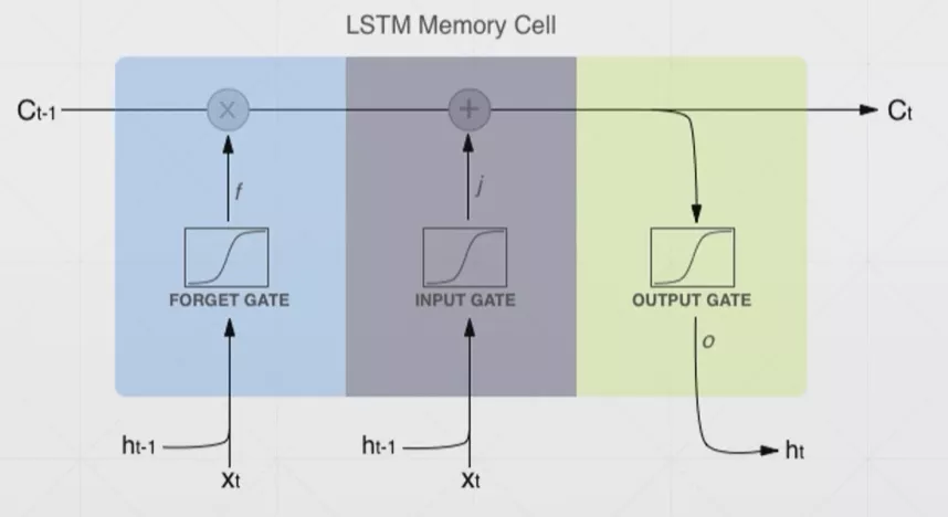
In [3]: from torch import nn
In [4]: lstm=nn.LSTM(input_size=100, hidden_size=20, num_layers=4)
In [5]: lstm
Out[5]: LSTM(100, 20, num_layers=4)
In [6]: x=torch.randn(10,3,100)
In [7]: out,(h,c)=lstm(x)
In [8]: out.shape,h.shape,c.shape
Out[8]: (torch.Size([10, 3, 20]), torch.Size([4, 3, 20]), torch.Size([4, 3, 20]))

其实和原来的RNN使用差别不是非常大

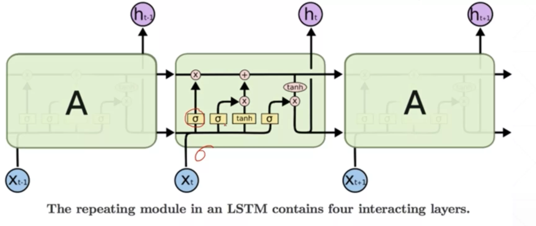
`nn.LSTMCell`

`init()`

和nn.LSTM初始化操作一样:

nn.LSTM(input_size,hidden_size,num_layers)

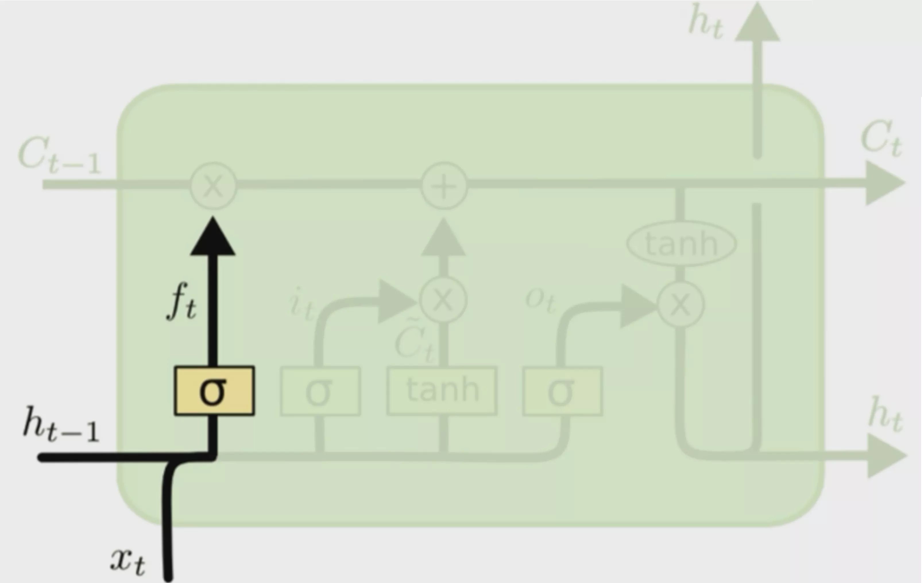
`LSTMCell.forward()`

1	ht,ct=lstmcell(xt,[ht_1,ct_1])

对于一个输入是[10,3,100]的数据，使用上述方法需要送入10次，每次送入大小是[3,100]

同理，相比LSTM，LSTMCell更加的灵活，我们更推荐这样的方式

同上，下面还是简单给出一个例子，帮助理解：

In [3]: from torch import nn
In [4]: xt=torch.randn(10,3,100)
In [5]: cell1=nn.LSTMCell(input_size=100,hidden_size=30)
In [6]: cell2=nn.LSTMCell(input_size=30,hidden_size=20)
In [7]: h1=torch.zeros(3,30)
In [8]: c1=torch.zeros(3,30)
In [9]: h2=torch.zeros(3,20)
In [10]: c2=torch.zeros(3,20)
In [11]: for x in xt:
    ...:     h1,c1=cell1(x,[h1,c1])
    ...:     h2,c2=cell2(h1,[h2,c2])
    
In [12]: h2.shape,c2.shape
Out[12]: (torch.Size([3, 20]), torch.Size([3, 20]))

LSTM情感分类实战

安利：Google CoLab

免费12H训练
免费K80GPU

界面类似Jupyter，我们只需要把我们的代码扔上去就可以跑啦。

数据导入

TEXT = data.Field(tokenize='spacy')
LABEL = data.LabelField(dtype=torch.float)
train_data, test_data = datasets.IMDB.splits(TEXT, LABEL)
print('len of train data:', len(train_data))
print('len of test data:', len(test_data))

运行结果

1 2	len of train data: 25000 len of test data: 25000

打出数据中的一个example进行观察

1 2	print(train_data.examples[15].text) print(train_data.examples[15].label)

1
2

['Well', 'when', 'watching', 'this', 'film', 'late', 'one', 'night', 'I', 'was', 'simple', 'amazed', 'by', 'it', "'s", 'greatness', '.', 'Fantastic', 'script', ',', 'great', 'acting', ',', 'costumes', 'and', 'special', 'effects', ',', 'and', 'the', 'plot', 'twists', ',', 'wow', '!', '!', 'In', 'fact', 'if', 'you', 'can', 'see', 'the', 'ending', 'coming', 'you', 'should', 'become', 'a', 'writer', 'yourself.<br', '/><br', '/>Great', ',', 'I', 'would', 'recommend', 'this', 'film', 'to', 'anyone', ',', 'especially', 'if', 'I', 'don;t', 'like', 'them', 'much.<br', '/><br', '/>Terrific']
pos

使用GloVe对数据编码

# word2vec, glove
TEXT.build_vocab(train_data, max_size=10000, vectors='glove.6B.100d')
LABEL.build_vocab(train_data)


batchsz = 30
device = torch.device('cuda')
train_iterator, test_iterator = data.BucketIterator.splits(
    (train_data, test_data),
    batch_size = batchsz,
    device=device
)

网络设计※

class RNN(nn.Module):
    
    def __init__(self, vocab_size, embedding_dim, hidden_dim):
        """
        """
        super(RNN, self).__init__()
        
        # [0-10001] => [100]
        self.embedding = nn.Embedding(vocab_size, embedding_dim)
        # [100] => [256]
        self.rnn = nn.LSTM(embedding_dim, hidden_dim, num_layers=2, 
                           bidirectional=True, dropout=0.5)
        # [256*2] => [1]
        self.fc = nn.Linear(hidden_dim*2, 1)
        self.dropout = nn.Dropout(0.5)
        
        
    def forward(self, x):
        """
        x: [seq_len, b] vs [b, 3, 28, 28]
        """
        # [seq, b, 1] => [seq, b, 100]
        embedding = self.dropout(self.embedding(x))
        
        # output: [seq, b, hid_dim*2]
        # hidden/h: [num_layers*2, b, hid_dim]
        # cell/c: [num_layers*2, b, hid_di]
        output, (hidden, cell) = self.rnn(embedding)
        
        # [num_layers*2, b, hid_dim] => 2 of [b, hid_dim] => [b, hid_dim*2]
        hidden = torch.cat([hidden[-2], hidden[-1]], dim=1)
        
        # [b, hid_dim*2] => [b, 1]
        hidden = self.dropout(hidden)
        out = self.fc(hidden)
        
        return out

因为nn.LSTM采用的是双向bidirectional=True,因此后面全连接层的hidden_size要乘2。最后LSTM算出来的hidden部分，最后两层就是实际网络的最后一层，只不过是两个方向，所以维度上占了两层。

`vocab_size`表示的是有多少个单词，`embedding_dim`表示的是表示一个单词需要多长维度的向量。

最后一个dropout的引入是为了加强网络的鲁棒性而引入的。

训练部分

optimizer = optim.Adam(rnn.parameters(), lr=1e-3)
criteon = nn.BCEWithLogitsLoss().to(device)
rnn.to(device)

def binary_acc(preds, y):
    """
    get accuracy
    """
    preds = torch.round(torch.sigmoid(preds))
    correct = torch.eq(preds, y).float()
    acc = correct.sum() / len(correct)
    return acc

def train(rnn, iterator, optimizer, criteon):
    
    avg_acc = []
    rnn.train()
    
    for i, batch in enumerate(iterator):
        
        # [seq, b] => [b, 1] => [b]
        pred = rnn(batch.text).squeeze(1) # 将第一个维度的信息压缩掉
        # 
        loss = criteon(pred, batch.label)
        acc = binary_acc(pred, batch.label).item()
        avg_acc.append(acc)
        
        optimizer.zero_grad()
        loss.backward()
        optimizer.step()
        
        if i%10 == 0:
            print(i, acc)
    # 一轮训练结束后打出训练过程中的平均准确率    
    avg_acc = np.array(avg_acc).mean()
    print('avg acc:', avg_acc)

eval部分

def eval(rnn, iterator, criteon):
    
    avg_acc = []
    
    rnn.eval() # 切换状态
    
    with torch.no_grad():
        for batch in iterator:

            # [b, 1] => [b]
            pred = rnn(batch.text).squeeze(1)

            #
            loss = criteon(pred, batch.label)

            acc = binary_acc(pred, batch.label).item()
            avg_acc.append(acc)
        
    avg_acc = np.array(avg_acc).mean()
    
    print('>>test:', avg_acc)

main部分

for epoch in range(10):
    
    eval(rnn, test_iterator, criteon)
    train(rnn, train_iterator, optimizer, criteon)

运行结果：

>>test: 0.4997602136050769
0 0.46666669845581055
10 0.40000003576278687
20 0.5
30 0.5
40 0.4333333671092987
50 0.5333333611488342
60 0.6000000238418579
70 0.5666667222976685
80 0.40000003576278687
90 0.36666667461395264
100 0.5333333611488342
110 0.6666666865348816
120 0.7333333492279053
130 0.4333333671092987
140 0.6000000238418579
150 0.5333333611488342
160 0.5
170 0.46666669845581055
180 0.6333333849906921
190 0.6666666865348816
200 0.40000003576278687
210 0.46666669845581055
220 0.5666667222976685
230 0.5
...
810 0.9666666984558105
820 0.9666666984558105
830 0.9666666984558105
avg acc: 0.9673461499545786

汇总

# -*- coding: utf-8 -*-
"""lstm

Automatically generated by Colaboratory.

Original file is located at
    https://colab.research.google.com/drive/1GX0Rqur8T45MSYhLU9MYWAbycfLH4-Fu
"""

!pip install torch
!pip install torchtext
!python -m spacy download en


# K80 gpu for 12 hours
import torch
from torch import nn, optim
from torchtext import data, datasets

print('GPU:', torch.cuda.is_available())

torch.manual_seed(123)

TEXT = data.Field(tokenize='spacy')
LABEL = data.LabelField(dtype=torch.float)
train_data, test_data = datasets.IMDB.splits(TEXT, LABEL)

print('len of train data:', len(train_data))
print('len of test data:', len(test_data))

print(train_data.examples[15].text)
print(train_data.examples[15].label)

# word2vec, glove
TEXT.build_vocab(train_data, max_size=10000, vectors='glove.6B.100d')
LABEL.build_vocab(train_data)


batchsz = 30
device = torch.device('cuda')
train_iterator, test_iterator = data.BucketIterator.splits(
    (train_data, test_data),
    batch_size = batchsz,
    device=device
)

class RNN(nn.Module):
    
    def __init__(self, vocab_size, embedding_dim, hidden_dim):
        """
        """
        super(RNN, self).__init__()
        
        # [0-10001] => [100]
        self.embedding = nn.Embedding(vocab_size, embedding_dim)
        # [100] => [256]
        self.rnn = nn.LSTM(embedding_dim, hidden_dim, num_layers=2, 
                           bidirectional=True, dropout=0.5)
        # [256*2] => [1]
        self.fc = nn.Linear(hidden_dim*2, 1)
        self.dropout = nn.Dropout(0.5)
        
        
    def forward(self, x):
        """
        x: [seq_len, b] vs [b, 3, 28, 28]
        """
        # [seq, b, 1] => [seq, b, 100]
        embedding = self.dropout(self.embedding(x))
        
        # output: [seq, b, hid_dim*2]
        # hidden/h: [num_layers*2, b, hid_dim]
        # cell/c: [num_layers*2, b, hid_di]
        output, (hidden, cell) = self.rnn(embedding)
        
        # [num_layers*2, b, hid_dim] => 2 of [b, hid_dim] => [b, hid_dim*2]
        hidden = torch.cat([hidden[-2], hidden[-1]], dim=1)
        
        # [b, hid_dim*2] => [b, 1]
        hidden = self.dropout(hidden)
        out = self.fc(hidden)
        
        return out

rnn = RNN(len(TEXT.vocab), 100, 256)

pretrained_embedding = TEXT.vocab.vectors
print('pretrained_embedding:', pretrained_embedding.shape)
rnn.embedding.weight.data.copy_(pretrained_embedding)
print('embedding layer inited.')

optimizer = optim.Adam(rnn.parameters(), lr=1e-3)
criteon = nn.BCEWithLogitsLoss().to(device)
rnn.to(device)

import numpy as np

def binary_acc(preds, y):
    """
    get accuracy
    """
    preds = torch.round(torch.sigmoid(preds))
    correct = torch.eq(preds, y).float()
    acc = correct.sum() / len(correct)
    return acc

def train(rnn, iterator, optimizer, criteon):
    
    avg_acc = []
    rnn.train()
    
    for i, batch in enumerate(iterator):
        
        # [seq, b] => [b, 1] => [b]
        pred = rnn(batch.text).squeeze(1)
        # 
        loss = criteon(pred, batch.label)
        acc = binary_acc(pred, batch.label).item()
        avg_acc.append(acc)
        
        optimizer.zero_grad()
        loss.backward()
        optimizer.step()
        
        if i%10 == 0:
            print(i, acc)
        
    avg_acc = np.array(avg_acc).mean()
    print('avg acc:', avg_acc)
    
    
def eval(rnn, iterator, criteon):
    
    avg_acc = []
    
    rnn.eval()
    
    with torch.no_grad():
        for batch in iterator:

            # [b, 1] => [b]
            pred = rnn(batch.text).squeeze(1)

            #
            loss = criteon(pred, batch.label)

            acc = binary_acc(pred, batch.label).item()
            avg_acc.append(acc)
        
    avg_acc = np.array(avg_acc).mean()
    
    print('>>test:', avg_acc)

for epoch in range(10):
    
    eval(rnn, test_iterator, criteon)
    train(rnn, train_iterator, optimizer, criteon)

PyTorch RNN&LSTM

序列表示（Sequence representation）

方法一

方法二

PyTorch实现

PyTorch 导入GloVe

RNN原理

RNN Layer使用

nn.RNN

forward

多层RNN

nn.RNNCell

初始化

使用方法

迭代操作

实战RNN波形预测

网络设计

训练部分

测试部分

代码汇总

结果

RNN训练问题

梯度爆炸

解决方法

PyTorch实现

梯度弥散

LSTM

三个Sigmoid

Forget gate

Input gate

更新C

Output gate

LSTM行为

LSTM解决梯度弥散

LSTM Layer

nn.LSTM

__init()__

LSTM.forward()

nn.LSTMCell

__init()__

LSTMCell.forward()

LSTM情感分类实战

安利：Google CoLab

数据导入

网络设计※

训练部分

eval部分

main部分

汇总

`nn.RNN`

`nn.RNNCell`

`nn.LSTM`

`init()`

`LSTM.forward()`

`nn.LSTMCell`

`init()`

`LSTMCell.forward()`