PyTorch：PyTorch终章：开GAN！

GAN简介

GAN的终极目的就是学习 $p(x)$ , $p(x)$ 是一个分布，比如它可以是二次元头像图片特征的分布，可以是一种类型的画作的特征集合，我们学会了 $p(x)$ 后，我们便可以在其中进行sample然后就可以进行创作了。这便是GAN的原理解释。

GAN 结构

生成器（Painter or Generator）
鉴别器（Critic or Discriminator）

GAN结构

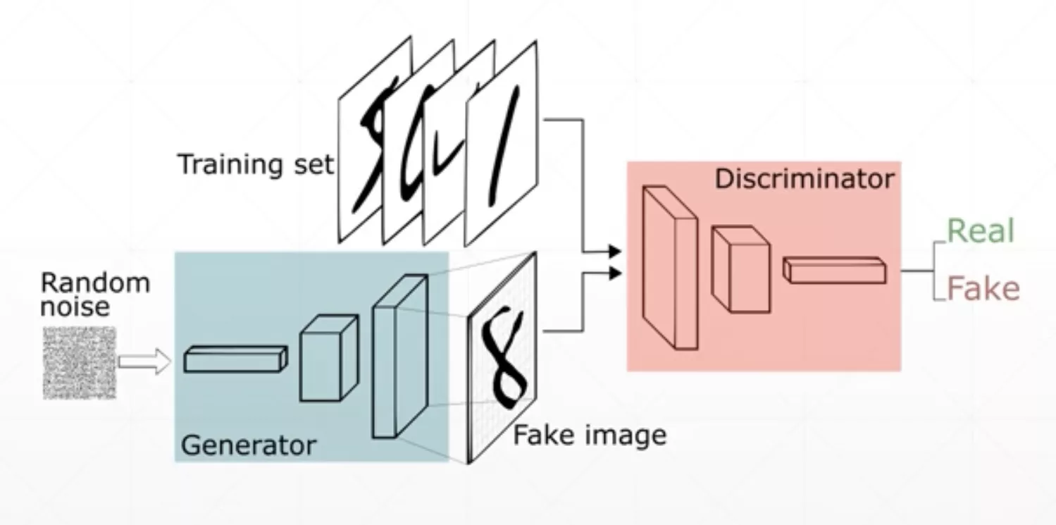
大致结构如上，生成器根据随机生成的信号，产生一幅“画”。鉴别器使用很多真的和假的“画”进行训练，来分辨画的真假，从而产生一个打分值。分值越高表明画越真实（鉴别器看来）。鉴别器的目标是尽可能的分辨出真“画”和假“画”。生成器的目标是尽可能的最大化鉴别器的打分（相当于尽可能的欺骗鉴别器）

GAN的出现让神经网络具有了创造性，当我们需要使用神经网络完成一些具有创造力的任务时，GAN是一个非常不错的选择。

这里推荐一个非常不错的关于GAN在线训练的网页链接

[GAN

playground: Experiment with Generative Adversarial Networks in your browser ](https://reiinakano.com/gan-playground/)

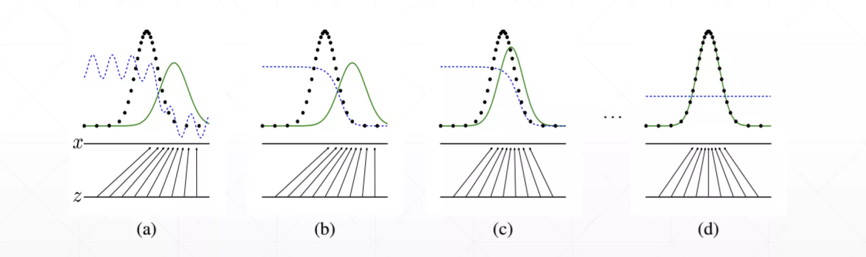
下图是GAN网络的形象解释，绿线是我们要学习的物体的特征（比如二次元头像的特征）的分布，黑线是我们学习到的特征的分布，蓝线是鉴别器的输出，一开始生成器和鉴别器都没有进行训练，所以生成器生成的分布非常的烂，鉴别器也无法很好的鉴别图片是否是生成器生成的（如图(a)所示），紧接着我们训练鉴别器，然后可以发现在训练一段时间后鉴别器已经可以很好的鉴别图片的真伪了（图b）。接着我们训练生成器，生成器的目标是尽量让鉴别器认为图片是真的，从而给出高分，随着训练次数的增加，生成器生成的分布会越来越接近真实的分布（如图©所示），在最后的时候连鉴别器也无法识别生成器生成图片的真伪时，训练结束。（图d）

GAN原理

GAN的训练分为两步。

固定生成器（G）训练鉴别器（D）使其收敛
固定鉴别器（D）训练生成器（G）使其收敛

下面我们就分别来详细说明一下这两步中的数学原理。

首先我们要明白我们的最终目标

\min\limits_{G}\max\limits_{D} L(D,G)=\mathbb{E}_{x\sim p_r(x)}[\log D(x)] + \mathbb{E}_{z\sim p_z(z)}[\log(1- D(G(z)))]

\min\limits_{G}\max\limits_{D} L(D,G)=\mathbb{E}_{x\sim p_r(x)}[\log D(x)] + \mathbb{E}_{x\sim p_g(x)}[\log(1- D(x))]

纳什均衡——D

对于固定的G，最好的D是：

D^*_G(x)=\frac{p_{data}(x)}{p_{data}(x)+p_g(x)}

训练D的准则（criterion）是对于给定的G最大化 $V(G,D)$

\begin{aligned} V(G,D) &= \int_x p_{data}(x)\log(D(x))dx + \int_z p(z)\log(1-D(g(z)))dz\\ &= \int_xp_{data}(x)\log(D(x))+p_g(x)\log(1-D(x))dx \end{aligned}

这个其实就是求期望，只是把它写成了积分形式。

我们对上面这个式子求导，就可以知道最好的 $D$ 是上面的 $D^*$

纳什均衡——G

当我们训练完D后，下面就轮到G进行训练了。

L(G,D^*)=2D_{JS}(p_r||p_g)-2\log2

这便是欺骗鉴别器这一直观理解的目标函数表达形式，我们的目的是最小化这个函数。

GAN的问题

训练稳定性差

导致这个情况主要是有两个原因：

数据本身的特征

因为在很多情况下 $P_G$ 和 $P_{data}$ 是几乎不可能重合的，因为这两个分布的特征是在高维特征空间中就几乎是两条线（仅用于说明），他们重合的部分几乎可以忽略。

几乎没有重合

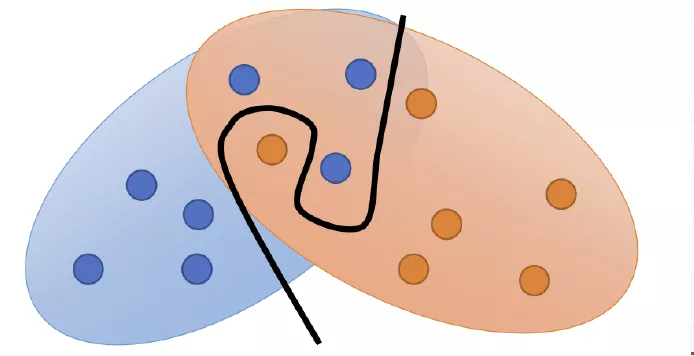
采样

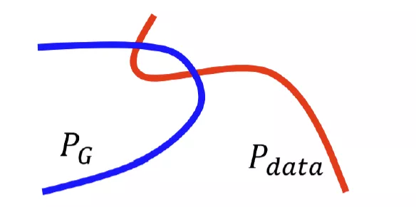
就算 $P_G$ 和 $P_{data}$ 还是有一部分重合的，但是如果我们采样没有采够的话，还是有可能出现下图的情况，让我们认为两个分布没有重合。（点为实际的采样点，两个椭圆表示的是实际的两个分布情况。）

采样不够的问题

JS

经过数学推导，只要两个分布不重叠，JS Divergence的取值永远都是 $\log 2$ 。这个就没有很好的量化分布之间距离的这种关系。而且根据数据的自然特性我们也知道这两个分布是不好重叠的，或者说大概率是不会重叠的，JS Divergence一直不变会给梯度下降带来很大的问题，导致模型一直不收敛。这便是JS Divergence在GAN中使用的一个非常严重的问题。

解决JS的问题

我们采用了Wasserstein Distance来代替JS。其根本思想就是衡量将一个分布变成另一个分布所需要的最小代价。（直观理解就是搬砖，把一个砖堆变成另外一种砖堆所需的最小代价）。

采用Wasserstein Distance来代替JS的GAN被称为WGAN

简要计算步骤如下图所示。

如何计算Wasserstein Distance

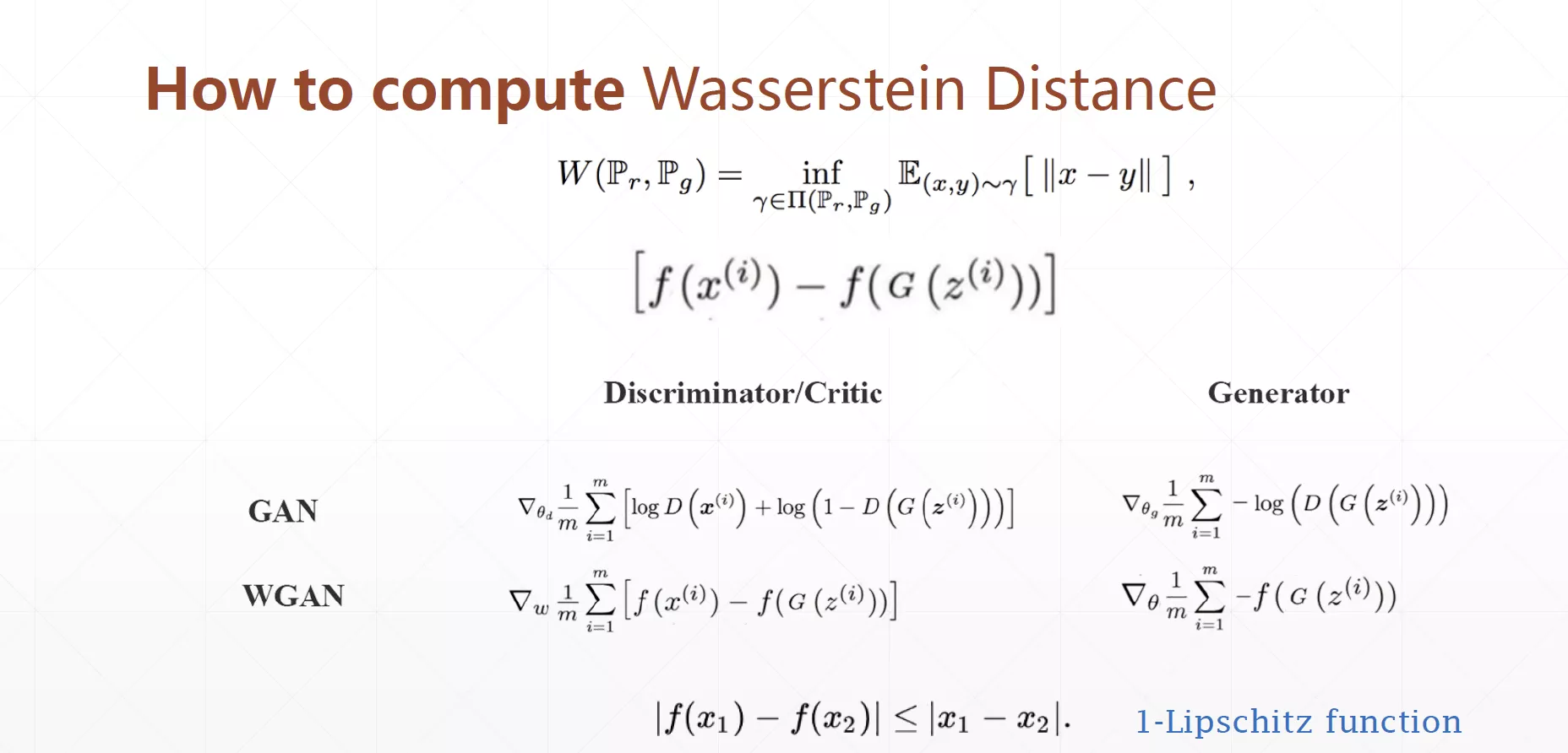
WGAN的提出从根本上解决了部分GAN无法收敛(训练不稳定)的问题。

实战GAN

网络结构

首先是建立网络结构，GAN的网络结构包含两个部分，一个是生成器（Generator），还有一个是鉴别器（Discriminator）。代码非常简答，这里就不再赘述了。

h_dim = 400
batchsz = 512

class Generator(nn.Module):

    def __init__(self):
        super(Generator, self).__init__()

        self.net = nn.Sequential(
            nn.Linear(2, h_dim),
            nn.ReLU(True),
            nn.Linear(h_dim, h_dim),
            nn.ReLU(True),
            nn.Linear(h_dim, h_dim),
            nn.ReLU(True),
            nn.Linear(h_dim, 2),
        )

    def forward(self, z):
        output = self.net(z)
        return output
    
class Discriminator(nn.Module):

    def __init__(self):
        super(Discriminator, self).__init__()

        self.net = nn.Sequential(
            nn.Linear(2, h_dim),
            nn.ReLU(True),
            nn.Linear(h_dim, h_dim),
            nn.ReLU(True),
            nn.Linear(h_dim, h_dim),
            nn.ReLU(True),
            nn.Linear(h_dim, 1),
            nn.Sigmoid()
        )

    def forward(self, x):
        output = self.net(x)
        return output.view(-1)

生成数据集

我们本次实验采用的数据集是统计学中经常使用的混合高斯模型，如下图所示，二维平面上一共是有8个高斯分布组合而成的一个混合分布图形。

混合高斯模型

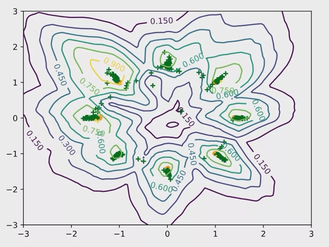
相信大家也明白了为什么输出是两个神经元——因为要在平面坐标系上进行可视化输出嘛😂

数据集生成代码如下：

def data_generator():
    '''
    8-gaussian mixture models
    :return:
    '''
    scale = 2.
    centers = [
        (1, 0),
        (-1, 0),
        (0, 1),
        (0, -1),
        (1. / np.sqrt(2), 1. / np.sqrt(2)),
        (1. / np.sqrt(2), -1. / np.sqrt(2)),
        (-1. / np.sqrt(2), 1. / np.sqrt(2)),
        (-1. / np.sqrt(2), -1. / np.sqrt(2))
    ]
    centers = [(scale * x, scale * y) for x, y in centers]
    while True:
        dataset = []
        for i in range(batchsz):
            point = np.random.randn(2) * .02
            center = random.choice(centers)
            point[0] += center[0]
            point[1] += center[1]
            dataset.append(point)
        dataset = np.array(dataset, dtype='float32')
        dataset /= 1.414  # stdev
        yield dataset

`yield`

这里大家可能好奇yield是干什么的，下面我举两个例子帮助大家理解。

以下关于yield的部分讲解转载自:https://blog.csdn.net/mieleizhi0522/article/details/82142856

例一

def dataset_generator():
    i=0
    while True:
        i=i+1
        yield i

if __name__ == '__main__':
    g = dataset_generator()
    
    for ii in range (10):
        print(next(g))
        print("*"*20)

代码运行结果是：

1
********************
2
********************
3
********************
4
********************
5
********************
6
********************
7
********************
8
********************
9
********************
10
********************

例二

def foo():
    print("starting...")
    while True:
        res = yield 4
        print("res:",res)
if __name__ == '__main__':        
    g = foo()
    print('ok')
    print(next(g))
    print("*"*20)
    print(next(g))

代码运行结果是：

ok
starting...
4
********************
res: None
4

到这里你可能就明白yield和return的关系和区别了，带yield的函数是一个生成器，而不是一个函数了，这个生成器有一个函数就是next函数，next就相当于“下一步”生成哪个数，这一次的next开始的地方是接着上一次的next停止的地方执行的，所以调用next的时候，生成器并不会从foo函数的开始执行，只是接着上一步停止的地方开始，然后遇到yield后，return出要生成的数，此步就结束。

训练部分

GAN的训练和其他神经网络的训练还有一点不太一样，GAN的训练是D和G分开训练，D先训练几轮后，定住D训练G，然后依次往复。有点像左脚踩右脚，原地升天那种感觉。

训练D

训练鉴别器分为三个部分，训练真实数据，训练假数据（G生成的），反向传播，首先是我们先给鉴别器输入真实的数据（代码中是xr，使用刚才我们写的data_generator生成）,鉴别器的输出是predr。我们的目标是最大化这一部分的输出（相当于最小化predr的相反数）。因此lossr = - (predr.mean())。然后我们再给鉴别器输入G生成的数据（代码中是xf）,鉴别器的输出是predf。我们的目标是最小化这一部分的输出（相当于最小化predr的相反数）。因此lossf = (predr.mean())。

# 1. train discriminator for k steps
for _ in range(5):
    x = next(data_iter)
    xr = torch.from_numpy(x).cuda()

    # [b]
    predr = (D(xr))
    # max log(lossr)
    lossr = - (predr.mean())

    # [b, 2]
    z = torch.randn(batchsz, 2).cuda()
    # stop gradient on G
    # [b, 2]
    xf = G(z).detach()
    # [b]
    predf = (D(xf))
    # min predf
    lossf = (predf.mean())

    # gradient penalty
    gp = gradient_penalty(D, xr, xf)

    loss_D = lossr + lossf + gp
    optim_D.zero_grad()
    loss_D.backward()
    # for p in D.parameters():
    #     print(p.grad.norm())
    optim_D.step()

注意：代码中有一句`xf

= G(z).detach()。这句话的作用是断开G和D之间相连的反向传播链，这样就不会再我们更新D的时候同时更新前面D的参数。详细解释： tensor.detach()返回一个新的tensor，从当前计算图中分离下来。但是仍指向原变量的存放位置，不同之处只是requirse_grad为false.得到的这个tensir永远不需要计算器梯度，不具有grad. 即使之后重新将它的requires_grad置为true,它也不会具有梯度grad.这样我们就会继续使用这个新的tensor进行计算，后面当我们进行反向传播时到该调用detach()的tensor就会停止，不能再继续向前进行传播. 注意：是继续使用这个新的tensor`进行计算！

训练G

然后接下来就是训练生成器G了，生成器的训练是根据随机正态分布中的采样来学习我们要学习的分布的特征。

# 2. train Generator
optim_D.zero_grad()
z = torch.randn(batchsz, 2).cuda()
xf = G(z)
predf = (D(xf))
# max predf
loss_G = - (predf.mean())
optim_G.zero_grad()
loss_G.backward()
optim_G.step()

注意：D训练完了以后一定要清零，防止G更新的时候反向传播更新D的网络参数。

结果

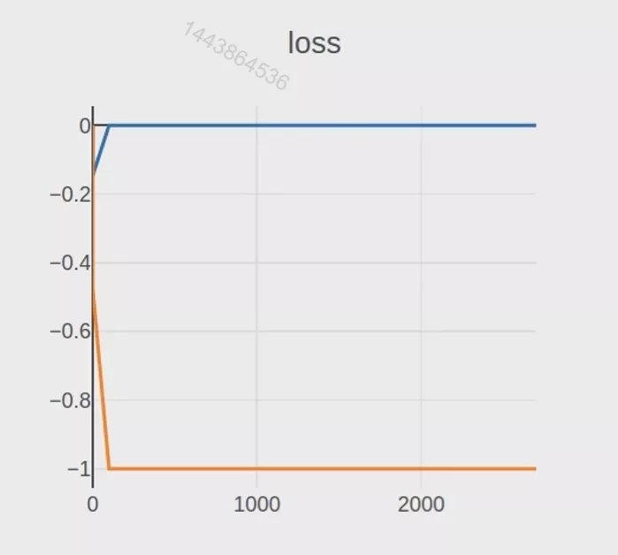
运行上面的代码，我们大概率得到的GAN的训练结果如下图所示，我们会发现D的鉴别很准确，误差是0，而G因为生成的很烂所以是-1，但是又因为JS的特性，导致模型无法更新（分布不重合，JS恒定，梯度为0）。因此为了解决这种问题我们需要引入上文所说的WGAN。

蓝线是Discriminator，黄线是Generator

实战WGAN

略微不同于GAN，主要是训练鉴别器部分有一些差别。训练鉴别器在WGAN中分为四个部分，训练真实数据，训练假数据（G生成的），梯度惩罚（gradient penalty），反向传播，首先是我们先给鉴别器输入真实的数据（代码中是xr，使用刚才我们写的data_generator生成）,鉴别器的输出是predr。我们的目标是最大化这一部分的输出（相当于最小化predr的相反数）。因此lossr = - (predr.mean())。然后我们再给鉴别器输入G生成的数据（代码中是xf）,鉴别器的输出是predf。我们的目标是最小化这一部分的输出（相当于最小化predr的相反数）。因此lossf = (predr.mean())。

然后接着是梯度惩罚操作，这一步非常重要后面我们单独讲，算出需要我们最小化的gp。然后我们就可以写出我们最后需要最小化的函数loss_D = lossr + lossf + gp。然后进行最后一步反向传播。

网络结构

和GAN基本一样，不再赘述。

相比于GAN只是多了一个**梯度惩罚(gradient_penalty)**部分。

梯度惩罚(gradient_penalty)

稍微理解一下即可，我们最后是要最小化该函数返回的gp的，具体代码如下所示：

def gradient_penalty(D, xr, xf):
    """

    :param D:
    :param xr:
    :param xf:
    :return:
    """
    LAMBDA = 0.3

    # only constrait for Discriminator
    xf = xf.detach()
    xr = xr.detach()

    # [b, 1] => [b, 2]
    alpha = torch.rand(batchsz, 1).cuda()
    alpha = alpha.expand_as(xr)

    interpolates = alpha * xr + ((1 - alpha) * xf)
    interpolates.requires_grad_()

    disc_interpolates = D(interpolates)

    gradients = autograd.grad(outputs=disc_interpolates, inputs=interpolates,
                              grad_outputs=torch.ones_like(disc_interpolates),
                              create_graph=True, retain_graph=True, only_inputs=True)[0] # 对中间点鉴别结果关于中间点信息求导

    gp = ((gradients.norm(2, dim=1) - 1) ** 2).mean() * LAMBDA

    return gp

外面调用如下代码所示：

1 2	# gradient penalty gp = gradient_penalty(D, xr, xf)

注意：这里的xf在前面是经过了detach()操作的。

代码汇总

最后在加上一些细节，最终的WGAN代码如下：

import  torch 
from    torch import nn, optim, autograd
import  numpy as np
import  visdom
from    torch.nn import functional as F
from    matplotlib import pyplot as plt
import  random

h_dim = 400
batchsz = 512
viz = visdom.Visdom()

class Generator(nn.Module):

    def __init__(self):
        super(Generator, self).__init__()

        self.net = nn.Sequential(
            nn.Linear(2, h_dim),
            nn.ReLU(True),
            nn.Linear(h_dim, h_dim),
            nn.ReLU(True),
            nn.Linear(h_dim, h_dim),
            nn.ReLU(True),
            nn.Linear(h_dim, 2),
        )

    def forward(self, z):
        output = self.net(z)
        return output


class Discriminator(nn.Module):

    def __init__(self):
        super(Discriminator, self).__init__()

        self.net = nn.Sequential(
            nn.Linear(2, h_dim),
            nn.ReLU(True),
            nn.Linear(h_dim, h_dim),
            nn.ReLU(True),
            nn.Linear(h_dim, h_dim),
            nn.ReLU(True),
            nn.Linear(h_dim, 1),
            nn.Sigmoid()
        )

    def forward(self, x):
        output = self.net(x)
        return output.view(-1)

def data_generator():

    scale = 2.
    centers = [
        (1, 0),
        (-1, 0),
        (0, 1),
        (0, -1),
        (1. / np.sqrt(2), 1. / np.sqrt(2)),
        (1. / np.sqrt(2), -1. / np.sqrt(2)),
        (-1. / np.sqrt(2), 1. / np.sqrt(2)),
        (-1. / np.sqrt(2), -1. / np.sqrt(2))
    ]
    centers = [(scale * x, scale * y) for x, y in centers]
    while True:
        dataset = []
        for i in range(batchsz):
            point = np.random.randn(2) * .02
            center = random.choice(centers)
            point[0] += center[0]
            point[1] += center[1]
            dataset.append(point)
        dataset = np.array(dataset, dtype='float32')
        dataset /= 1.414  # stdev
        yield dataset

    # for i in range(100000//25):
    #     for x in range(-2, 3):
    #         for y in range(-2, 3):
    #             point = np.random.randn(2).astype(np.float32) * 0.05
    #             point[0] += 2 * x
    #             point[1] += 2 * y
    #             dataset.append(point)
    #
    # dataset = np.array(dataset)
    # print('dataset:', dataset.shape)
    # viz.scatter(dataset, win='dataset', opts=dict(title='dataset', webgl=True))
    #
    # while True:
    #     np.random.shuffle(dataset)
    #
    #     for i in range(len(dataset)//batchsz):
    #         yield dataset[i*batchsz : (i+1)*batchsz]


def generate_image(D, G, xr, epoch):
    """
    Generates and saves a plot of the true distribution, the generator, and the
    critic.
    """
    N_POINTS = 128
    RANGE = 3
    plt.clf()

    points = np.zeros((N_POINTS, N_POINTS, 2), dtype='float32')
    points[:, :, 0] = np.linspace(-RANGE, RANGE, N_POINTS)[:, None]
    points[:, :, 1] = np.linspace(-RANGE, RANGE, N_POINTS)[None, :]
    points = points.reshape((-1, 2))
    # (16384, 2)
    # print('p:', points.shape)

    # draw contour
    with torch.no_grad():
        points = torch.Tensor(points).cuda() # [16384, 2]
        disc_map = D(points).cpu().numpy() # [16384]
    x = y = np.linspace(-RANGE, RANGE, N_POINTS)
    cs = plt.contour(x, y, disc_map.reshape((len(x), len(y))).transpose())
    plt.clabel(cs, inline=1, fontsize=10)
    # plt.colorbar()


    # draw samples
    with torch.no_grad():
        z = torch.randn(batchsz, 2).cuda() # [b, 2]
        samples = G(z).cpu().numpy() # [b, 2]
    plt.scatter(xr[:, 0], xr[:, 1], c='orange', marker='.')
    plt.scatter(samples[:, 0], samples[:, 1], c='green', marker='+')

    viz.matplot(plt, win='contour', opts=dict(title='p(x):%d'%epoch))


def weights_init(m):
    if isinstance(m, nn.Linear):
        # m.weight.data.normal_(0.0, 0.02)
        nn.init.kaiming_normal_(m.weight)
        m.bias.data.fill_(0)

def gradient_penalty(D, xr, xf):
    """

    :param D:
    :param xr:
    :param xf:
    :return:
    """
    LAMBDA = 0.3

    # only constrait for Discriminator
    xf = xf.detach()
    xr = xr.detach()

    # [b, 1] => [b, 2]
    alpha = torch.rand(batchsz, 1).cuda()
    alpha = alpha.expand_as(xr)

    interpolates = alpha * xr + ((1 - alpha) * xf)
    interpolates.requires_grad_()

    disc_interpolates = D(interpolates)

    gradients = autograd.grad(outputs=disc_interpolates, inputs=interpolates,
                              grad_outputs=torch.ones_like(disc_interpolates),
                              create_graph=True, retain_graph=True, only_inputs=True)[0]

    gp = ((gradients.norm(2, dim=1) - 1) ** 2).mean() * LAMBDA

    return gp

def main():

    torch.manual_seed(23)
    np.random.seed(23)

    G = Generator().cuda()
    D = Discriminator().cuda()
    G.apply(weights_init)
    D.apply(weights_init)

    optim_G = optim.Adam(G.parameters(), lr=1e-3, betas=(0.5, 0.9))
    optim_D = optim.Adam(D.parameters(), lr=1e-3, betas=(0.5, 0.9))


    data_iter = data_generator()
    print('batch:', next(data_iter).shape)

    viz.line([[0,0]], [0], win='loss', opts=dict(title='loss',
                                                 legend=['D', 'G']))

    for epoch in range(50000):

        # 1. train discriminator for k steps
        for _ in range(5):
            x = next(data_iter)
            xr = torch.from_numpy(x).cuda()

            # [b]
            predr = (D(xr))
            # max log(lossr)
            lossr = - (predr.mean())

            # [b, 2]
            z = torch.randn(batchsz, 2).cuda()
            # stop gradient on G
            # [b, 2]
            xf = G(z).detach()
            # [b]
            predf = (D(xf))
            # min predf
            lossf = (predf.mean())

            # gradient penalty
            gp = gradient_penalty(D, xr, xf)

            loss_D = lossr + lossf + gp
            optim_D.zero_grad()
            loss_D.backward()
            # for p in D.parameters():
            #     print(p.grad.norm())
            optim_D.step()


        # 2. train Generator
        optim_D.zero_grad()
        z = torch.randn(batchsz, 2).cuda()
        xf = G(z)
        predf = (D(xf))
        # max predf
        loss_G = - (predf.mean())
        optim_G.zero_grad()
        loss_G.backward()
        optim_G.step()


        if epoch % 100 == 0:
            viz.line([[loss_D.item(), loss_G.item()]], [epoch], win='loss', update='append')

            generate_image(D, G, xr, epoch)

            print(loss_D.item(), loss_G.item())






if __name__ == '__main__':
    main()