PyTorch - 教程合集
个人PyTorch学习过程中整理归纳的教程,适合入门学习使用✨

简介

因为课程需要学习PyTorch,所以这里就先简单的入个门,使用PyTorch实现一个简单的3层BP全连接神经网络实验。实验使用的数据集是MNIST手写数字识别数据集。

MNIST手写数据集

我们设计的网络结构是4层全连接神经网络,因为一个数字所存储的像素信息是28×28×128\times 28\times 1因此,网络的第一层有28×28×1=78428\times 28 \times 1=784个神经元,第二层设计的有 256个神经元,第三层有64个神经元,第四层有10个神经元。其中第一层和第二层,第二层和第三层,第三层和第四层之间,都有一个relu激活函数。最后第四层的1×101\times 10输出向量相当于是对10个数字的识别相似度,最大的数的index代表识别出来相似度最高的数字。

网络构建部分的代码实现如下:

1
2
3
4
5
6
7
8
9
10
11
12
13
14
15
16
17
18
19
20
class Net(nn.Module):

def __init__(self):
super(Net, self).__init__()

# xw+b
self.fc1 = nn.Linear(28*28, 256)
self.fc2 = nn.Linear(256, 64)
self.fc3 = nn.Linear(64, 10)

def forward(self, x):
# x: [b, 1, 28, 28]
# h1 = relu(xw1+b1)
x = F.relu(self.fc1(x))
# h2 = relu(h1w2+b2)
x = F.relu(self.fc2(x))
# h3 = h2w3+b3
x = self.fc3(x)

return x

定义损失函数是:

cost=(predY)2cost=\sum(pred-Y)^2

代码实现与讲解

数据载入

1
2
3
4
5
6
7
8
9
10
11
12
13
14
15
16
17
18
19
20
21
22
23
24
25
26
27
28
29
30
31
32
33
34
35
36
import  torch
from torch import nn
from torch.nn import functional as F
from torch import optim

import torchvision
from matplotlib import pyplot as plt

from utils import plot_image, plot_curve, one_hot


batch_size = 512 #批

# step1. load dataset
train_loader = torch.utils.data.DataLoader(
torchvision.datasets.MNIST('mnist_data', train=True, download=True,
transform=torchvision.transforms.Compose([
torchvision.transforms.ToTensor(),
torchvision.transforms.Normalize(
(0.1307,), (0.3081,))
])),
batch_size=batch_size, shuffle=True)

test_loader = torch.utils.data.DataLoader(
torchvision.datasets.MNIST('mnist_data/', train=False, download=True,
transform=torchvision.transforms.Compose([
torchvision.transforms.ToTensor(),
torchvision.transforms.Normalize(
(0.1307,), (0.3081,))
])),
batch_size=batch_size, shuffle=False)

x, y = next(iter(train_loader))
print(x.shape, y.shape, x.min(), x.max())
plot_image(x, y, 'image sample')

这里就是载入了训练集train_loadertest_loader

然后倒数第三行的next返回的是训练集中下一个元素(下一个batch),因为是batch大小是512,所以print出来的x和y的维度如下所示。

1
torch.Size([512, 1, 28, 28]) torch.Size([512]) tensor(-0.4242) tensor(2.8215)

建立网络

上面已经进行过讲解了,这里不再赘述

1
2
3
4
5
6
7
8
9
10
11
12
13
14
15
16
17
18
19
20
class Net(nn.Module):

def __init__(self):
super(Net, self).__init__()

# xw+b
self.fc1 = nn.Linear(28*28, 256)
self.fc2 = nn.Linear(256, 64)
self.fc3 = nn.Linear(64, 10)

def forward(self, x):
# x: [b, 1, 28, 28]
# h1 = relu(xw1+b1)
x = F.relu(self.fc1(x))
# h2 = relu(h1w2+b2)
x = F.relu(self.fc2(x))
# h3 = h2w3+b3
x = self.fc3(x)

return x

初始化参数

1
2
3
net = Net() # 实例化对象,这里就是我们建立的网络
# [w1, b1, w2, b2, w3, b3]
optimizer = optim.SGD(net.parameters(), lr=0.01, momentum=0.9) # 初始化参数(设置超参数和随机初始化参数)

开始训练

1
2
3
4
5
6
7
8
9
10
11
12
13
14
15
16
17
18
19
20
21
22
23
for epoch in range(3):

for batch_idx, (x, y) in enumerate(train_loader):

# x: [b, 1, 28, 28], y: [512]
# [b, 1, 28, 28] => [b, 784]
x = x.view(x.size(0), 28*28)
# => [b, 10]
out = net(x)
# [b, 10]
y_onehot = one_hot(y)
# loss = mse(out, y_onehot)
loss = F.mse_loss(out, y_onehot)

optimizer.zero_grad()
loss.backward()
# w' = w - lr*grad
optimizer.step()

train_loss.append(loss.item())

if batch_idx % 10==0:
print(epoch, batch_idx, loss.item())

epoch代表训练的轮数,这里一共训练三轮。然后每一轮中每次训练取出同一batch下的所有训练数据(一共512组),注释中的b=512

然后先进行reshape。代码中的view实现的功能类似numpy中reshape。这里就将X从一个四维数组512×1×28×28512\times 1 \times 28\times 28转化为了512×784512 \times 784的二维数组。然后扔入网络进行训练,将y标签先转化为独热编码和网络扔出的值结合计算loss。计算结束后就进行以下三步:

1
2
3
4
optimizer.zero_grad() # 将模型的参数梯度初始化为0
loss.backward() # 反向传播计算梯度
# w' = w - lr*grad
optimizer.step() # 更新所有参数

总结一下,训练过程的代码一般就以下几块:

1
2
3
4
5
6
7
8
9
10
optimizer.zero_grad()                       # 将模型的参数梯度初始化为0

outputs=model(inputs) # 前向传播计算预测值

loss = cost(outputs, y_train) # 计算当前损失

loss.backward() # 反向传播计算梯度

optimizer.step() # 更新所有参数

然后训练过程就结束了,下面就是测试环节了。

进行测试

1
2
3
4
5
6
7
8
9
10
11
12
13
14
15
16
17
total_correct = 0
for x,y in test_loader:
x = x.view(x.size(0), 28*28)
out = net(x)
# out: [b, 10] => pred: [b]
pred = out.argmax(dim=1)
correct = pred.eq(y).sum().float().item()
total_correct += correct

total_num = len(test_loader.dataset)
acc = total_correct / total_num
print('test acc:', acc)

x, y = next(iter(test_loader))
out = net(x.view(x.size(0), 28*28))
pred = out.argmax(dim=1)
plot_image(x, pred, 'test')

同理,和训练过程很像,也是先使用view,reshape一下后,扔入网络,得到out后,寻找数值最大的下标记录在pred中,pred就是测试预测的数值,然后就可以计算正确率等评价指标了。

总结

不同于tensorflow的place_holder,pytorch网络定义更加简单便捷,只需要使用类似nn.Linear(a,b)的函数定义连接方式,然后最后实例化网络的时候传入一个parameter()就可以了,相比于tensorflow确实更加简单。

最终代码

mnist_train.py

1
2
3
4
5
6
7
8
9
10
11
12
13
14
15
16
17
18
19
20
21
22
23
24
25
26
27
28
29
30
31
32
33
34
35
36
37
38
39
40
41
42
43
44
45
46
47
48
49
50
51
52
53
54
55
56
57
58
59
60
61
62
63
64
65
66
67
68
69
70
71
72
73
74
75
76
77
78
79
80
81
82
83
84
85
86
87
88
89
90
91
92
93
94
95
96
97
98
99
100
101
102
103
104
105
106
107
108
109
110
111
112
113
114
import  torch
from torch import nn
from torch.nn import functional as F
from torch import optim

import torchvision
from matplotlib import pyplot as plt

from utils import plot_image, plot_curve, one_hot


batch_size = 512 #批

# step1. load dataset
train_loader = torch.utils.data.DataLoader(
torchvision.datasets.MNIST('mnist_data', train=True, download=True,
transform=torchvision.transforms.Compose([
torchvision.transforms.ToTensor(),
torchvision.transforms.Normalize(
(0.1307,), (0.3081,))
])),
batch_size=batch_size, shuffle=True)

test_loader = torch.utils.data.DataLoader(
torchvision.datasets.MNIST('mnist_data/', train=False, download=True,
transform=torchvision.transforms.Compose([
torchvision.transforms.ToTensor(),
torchvision.transforms.Normalize(
(0.1307,), (0.3081,))
])),
batch_size=batch_size, shuffle=False)

x, y = next(iter(train_loader))
print(x.shape, y.shape, x.min(), x.max())
plot_image(x, y, 'image sample')


class Net(nn.Module):

def __init__(self):
super(Net, self).__init__()

# xw+b
self.fc1 = nn.Linear(28*28, 256)
self.fc2 = nn.Linear(256, 64)
self.fc3 = nn.Linear(64, 10)

def forward(self, x):
# x: [b, 1, 28, 28]
# h1 = relu(xw1+b1)
x = F.relu(self.fc1(x))
# h2 = relu(h1w2+b2)
x = F.relu(self.fc2(x))
# h3 = h2w3+b3
x = self.fc3(x)

return x


net = Net()
# [w1, b1, w2, b2, w3, b3]
optimizer = optim.SGD(net.parameters(), lr=0.01, momentum=0.9)


train_loss = []

for epoch in range(3):

for batch_idx, (x, y) in enumerate(train_loader):

# x: [b, 1, 28, 28], y: [512]
# [b, 1, 28, 28] => [b, 784]
x = x.view(x.size(0), 28*28)
# => [b, 10]
out = net(x)
# [b, 10]
y_onehot = one_hot(y)
# loss = mse(out, y_onehot)
loss = F.mse_loss(out, y_onehot)

optimizer.zero_grad()
loss.backward()
# w' = w - lr*grad
optimizer.step()

train_loss.append(loss.item())

if batch_idx % 10==0:
print(epoch, batch_idx, loss.item())

plot_curve(train_loss) # 画出损失函数
# we get optimal [w1, b1, w2, b2, w3, b3]


total_correct = 0
for x,y in test_loader:
x = x.view(x.size(0), 28*28)
out = net(x)
# out: [b, 10] => pred: [b]
pred = out.argmax(dim=1)
correct = pred.eq(y).sum().float().item()
total_correct += correct

total_num = len(test_loader.dataset)
acc = total_correct / total_num
print('test acc:', acc)

x, y = next(iter(test_loader))
out = net(x.view(x.size(0), 28*28))
pred = out.argmax(dim=1)
plot_image(x, pred, 'test')

utils.py

1
2
3
4
5
6
7
8
9
10
11
12
13
14
15
16
17
18
19
20
21
22
23
24
25
26
27
28
29
30
31
32
import  torch
from matplotlib import pyplot as plt


def plot_curve(data):
fig = plt.figure()
plt.plot(range(len(data)), data, color='blue')
plt.legend(['value'], loc='upper right')
plt.xlabel('step')
plt.ylabel('value')
plt.show()


def plot_image(img, label, name):

fig = plt.figure()
for i in range(6):
plt.subplot(2, 3, i + 1)
plt.tight_layout()
plt.imshow(img[i][0]*0.3081+0.1307, cmap='gray', interpolation='none')
plt.title("{}: {}".format(name, label[i].item()))
plt.xticks([])
plt.yticks([])
plt.show()


def one_hot(label, depth=10):
out = torch.zeros(label.size(0), depth)
idx = torch.LongTensor(label).view(-1, 1)
out.scatter_(dim=1, index=idx, value=1)
return out

结果

cmd输出

训练集

损失函数图

预测结果

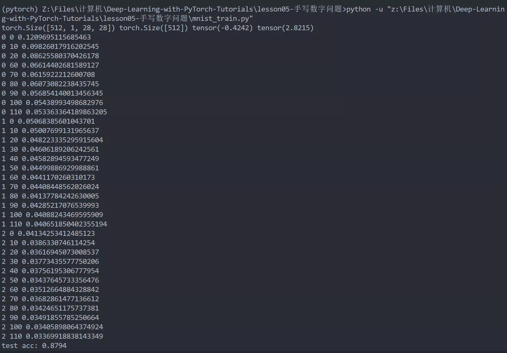
最终可以发现打印出来的均预测正确。acc为0.8794,是可以接受的正确率。


本站由 @anonymity 使用 Stellar 主题创建。
本博客所有文章除特别声明外,均采用 CC BY-NC-SA 4.0 许可协议,转载请注明出处。